| Type: | Package |
| Version: | 1.0.2 |
| Date: | 2025-12-09 |
| Title: | Bayesian Change-Point Detection and Time Series Decomposition |
| Author: | Tongxi Hu [aut], Yang Li [aut], Xuesong Zhang [aut], Kaiguang Zhao [aut, cre], Jack Dongarra [ctb], Cleve Moler [ctb] |
| Maintainer: | Kaiguang Zhao <zhao.1423@osu.edu> |
| Depends: | R (≥ 2.10.0),methods, utils |
| Description: | BEAST is a Bayesian estimator of abrupt change, seasonality, and trend for decomposing univariate time series and 1D sequential data. Interpretation of time series depends on model choice; different models can yield contrasting or contradicting estimates of patterns, trends, and mechanisms. BEAST alleviates this by abandoning the single-best-model paradigm and instead using Bayesian model averaging over many competing decompositions. It detects and characterizes abrupt changes (changepoints, breakpoints, structural breaks, joinpoints), cyclic or seasonal variation, and nonlinear trends. BEAST not only detects when changes occur but also quantifies how likely the changes are true. It estimates not just piecewise linear trends but also arbitrary nonlinear trends. BEAST is generically applicable to any real-valued time series, such as those from remote sensing, economics, climate science, ecology, hydrology, and other environmental and biological systems. Example applications include identifying regime shifts in ecological data, mapping forest disturbance and land degradation from satellite image time series, detecting market trends in economic indicators, pinpointing anomalies and extreme events in climate records, and analyzing system dynamics in biological time series. Details are given in Zhao et al. (2019) <doi:10.1016/j.rse.2019.04.034>. |
| LazyData: | true |
| Imports: | grid |
| License: | GPL-2 | GPL-3 [expanded from: GPL (≥ 2)] |
| URL: | https://github.com/zhaokg/Rbeast |
| NeedsCompilation: | yes |
| Packaged: | 2025-12-17 19:43:05 UTC; zhaokg |
| Repository: | CRAN |
| Date/Publication: | 2025-12-19 09:00:02 UTC |
DNA copy number alteration data in array-based CGH data for Chromesome 11
Description
CNAchrom11 is a vector of the log2 intensity ratios for cell line GM03576 for Chromosome 11, obtained from Snijders et al. (2001).
Usage
data(CNAchrom11)
Source
Snijders et al. (2001), Assembly of microarrays for genome-wide measurement of DNA copy number, Nature Genetics, 29, 263-264 (http://www.nature.com/ng/journal/v29/n3/full/ng754.html).
References
Zhao, K., Wulder, M.A., Hu, T., Bright, R., Wu, Q., Qin, H., Li, Y., Toman, E., Mallick, B., Zhang, X. and Brown, M., 2019. Detecting change-point, trend, and seasonality in satellite time series data to track abrupt changes and nonlinear dynamics: A Bayesian ensemble algorithm. Remote Sensing of Environment, 232, p.111181 (the beast algorithm paper).
Zhao, K., Valle, D., Popescu, S., Zhang, X. and Mallick, B., 2013. Hyperspectral remote sensing of plant biochemistry using Bayesian model averaging with variable and band selection. Remote Sensing of Environment, 132, pp.102-119 (the Bayesian MCMC scheme used in beast).
Hu, T., Toman, E.M., Chen, G., Shao, G., Zhou, Y., Li, Y., Zhao, K. and Feng, Y., 2021. Mapping fine-scale human disturbances in a working landscape with Landsat time series on Google Earth Engine. ISPRS Journal of Photogrammetry and Remote Sensing, 176, pp.250-261(a beast application paper).
Examples
 library(Rbeast)
 data(CNAchrom11)


 o = beast(CNAchrom11, season='none') # no periodic component
 plot(o)
30 years' AVHRR NDVI data at a Yellostone site
Description
Yellowstone is a vector comprising 30 years' AVHRR NDVI data at a Yellostone site
Usage
data(Yellowstone)
Source
Rbeast v0.9.2
References
Zhao, K., Wulder, M.A., Hu, T., Bright, R., Wu, Q., Qin, H., Li, Y., Toman, E., Mallick, B., Zhang, X. and Brown, M., 2019. Detecting change-point, trend, and seasonality in satellite time series data to track abrupt changes and nonlinear dynamics: A Bayesian ensemble algorithm. Remote Sensing of Environment, 232, p.111181 (the beast algorithm paper).
Zhao, K., Valle, D., Popescu, S., Zhang, X. and Mallick, B., 2013. Hyperspectral remote sensing of plant biochemistry using Bayesian model averaging with variable and band selection. Remote Sensing of Environment, 132, pp.102-119 (the Bayesian MCMC scheme used in beast).
Hu, T., Toman, E.M., Chen, G., Shao, G., Zhou, Y., Li, Y., Zhao, K. and Feng, Y., 2021. Mapping fine-scale human disturbances in a working landscape with Landsat time series on Google Earth Engine. ISPRS Journal of Photogrammetry and Remote Sensing, 176, pp.250-261(a beast application paper).
Examples
 library(Rbeast)
 data(Yellowstone)
 plot(Yellowstone,type='l')

 result=beast(Yellowstone)
 plot(result)
Bayesian changepoint detection and time series decomposition into trend, seasonality, and abrupt changes
Description
beast is a high-level interface to the BEAST algorithm, a Bayesian model averaging approach for decomposing regular time series or other 1D sequential data into individual components, including abrupt changes, trends, and periodic/seasonal variations. BEAST is useful for changepoint detection (e.g., breakpoints, joinpoints, or structural breaks), nonlinear trend analysis, time series decomposition, and time series segmentation.
Usage
beast(
  y,
  start          = 1,
  deltat         = 1,
  season         = c("harmonic", "svd", "dummy", "none"),
  period         = NULL,
  scp.minmax     = c(0, 10), sorder.minmax   = c(0, 5),
  tcp.minmax     = c(0, 10), torder.minmax   = c(0, 1),
  sseg.min       = NULL,     sseg.leftmargin = NULL, sseg.rightmargin = NULL,
  tseg.min       = NULL,     tseg.leftmargin = NULL, tseg.rightmargin = NULL,
  s.complexfct   = 0.0,
  t.complexfct   = 0.0,
  method         = c("bayes", "bic", "aic", "aicc", "hic",
                     "bic0.25", "bic0.5", "bic1.5", "bic2"),
  detrend        = FALSE,
  deseasonalize  = FALSE,
  mcmc.seed      = 0,
  mcmc.burnin    = 200,
  mcmc.chains    = 3,
  mcmc.thin      = 5,
  mcmc.samples   = 8000,
  precValue      = 1.5,
  precPriorType  = c("componentwise", "uniform", "constant", "orderwise"),
  hasOutlier     = FALSE,
  ocp.minmax     = c(0, 10),
  print.param    = TRUE,
  print.progress = TRUE,
  print.warning  = TRUE,
  quiet          = FALSE,
  dump.ci        = FALSE,
  dump.mcmc      = FALSE,
  gui            = FALSE,
  ...
)
Arguments
y |
If |
start |
|
deltat |
|
season |
Character (default
|
period |
Numeric or character string. The period of the seasonal/periodic component in
|
scp.minmax |
A numeric vector of length 2 (integers
|
sorder.minmax |
A numeric vector of length 2 (integers
|
tcp.minmax |
A numeric vector of length 2 (integers
|
torder.minmax |
A numeric vector of length 2 (integers
|
sseg.min |
An integer ( |
sseg.leftmargin |
Integer ( |
sseg.rightmargin |
Integer ( |
tseg.min |
Integer ( |
tseg.leftmargin |
Integer ( |
tseg.rightmargin |
Integer ( |
s.complexfct |
Numeric (default |
t.complexfct |
Numeric (default |
method |
Character (default
|
detrend |
Logical; if |
deseasonalize |
Logical; if |
mcmc.seed |
Integer ( |
mcmc.chains |
Integer ( |
mcmc.thin |
Integer ( |
mcmc.burnin |
Integer ( |
mcmc.samples |
Integer ( |
precValue |
Numeric ( |
precPriorType |
Character; one of
|
hasOutlier |
Logical; if
|
ocp.minmax |
Numeric vector of length 2 (integers |
print.param |
Logical; if |
print.progress |
Logical; if |
print.warning |
Logical; if |
quiet |
Logical; if |
dump.ci |
Logical; if |
dump.mcmc |
Logical; if |
gui |
Logical; if |
... |
Additional arguments reserved for future extensions and backward compatibility. Certain low-level settings are only available via |
Value
The result is an object of class "beast", i.e., a list with structure identical to the outputs of beast.irreg and beast123. The exact array dimensions depend on the input y. Below we assume a single time series input of length N.
time |
Numeric vector of length |
data |
A vector, matrix, or 3D array; a copy of the input |
marg_lik |
Numeric; the average marginal likelihood of the sampled models. Larger values indicate better fit for a given time series (e.g., |
R2 |
Numeric; coefficient of determination (R-squared) of the fitted model. |
RMSE |
Numeric; root mean squared error of the fitted model. |
sig2 |
Numeric; estimated variance of the residual error. |
trend |
|
season |
|
outlier |
|
Note
The three functions beast(), beast.irreg(), and beast123() implement the same BEAST algorithm but with different APIs. There is a one-to-one correspondence between (1) the arguments of beast() / beast.irreg() and (2) the metadata, prior, mcmc, and extra lists used by beast123(). Examples include:
start | <-> | metadata$startTime |
deltat | <-> | metadata$deltaTime |
deseasonalize | <-> | metadata$deseasonalize |
hasOutlier | <-> | metadata$hasOutlier |
scp.minmax[1:2] | <-> | prior$seasonMinKnotNum, prior$seasonMaxKnotNum |
sorder.minmax[1:2] | <-> | prior$seasonMinOrder, prior$seasonMaxOrder |
sseg.min | <-> | prior$seasonMinSepDist |
tcp.minmax[1:2] | <-> | prior$trendMinKnotNum, prior$trendMaxKnotNum |
torder.minmax[1:2] | <-> | prior$trendMinOrder, prior$trendMaxOrder |
tseg.leftmargin | <-> | prior$trendLeftMargin |
tseg.rightmargin | <-> | prior$trendRightMargin |
s.complexfct | <-> | prior$seasonComplexityFactor |
t.complexfct | <-> | prior$trendComplexityFactor |
mcmc.seed | <-> | mcmc$seed |
dump.ci | <-> | extra$computeCredible.
|
For large data sets, irregular time series, or stacked images, beast123() is generally the recommended interface.
References
Zhao, K., Wulder, M.A., Hu, T., Bright, R., Wu, Q., Qin, H., Li, Y., Toman, E., Mallick, B., Zhang, X. and Brown, M., 2019. Detecting change-point, trend, and seasonality in satellite time series data to track abrupt changes and nonlinear dynamics: A Bayesian ensemble algorithm. Remote Sensing of Environment, 232, p.111181 (the beast algorithm paper).
Zhao, K., Valle, D., Popescu, S., Zhang, X. and Mallick, B., 2013. Hyperspectral remote sensing of plant biochemistry using Bayesian model averaging with variable and band selection. Remote Sensing of Environment, 132, pp.102-119 (the Bayesian MCMC scheme used in beast).
Hu, T., Toman, E.M., Chen, G., Shao, G., Zhou, Y., Li, Y., Zhao, K. and Feng, Y., 2021. Mapping fine-scale human disturbances in a working landscape with Landsat time series on Google Earth Engine. ISPRS Journal of Photogrammetry and Remote Sensing, 176, pp.250-261(a beast application paper).
See Also
beast.irreg,
beast123,
minesweeper,
tetris,
geeLandsat
Examples
library(Rbeast)
#------------------------------------Example 1----------------------------------------#
# 'googletrend_beach' is the monthly Google Trends popularity of searching for 'beach'
# in the US from 2004 to 2022. Sudden changes coincide with known extreme weather
# events (e.g., 2006 North American Blizzard, 2011 record US summer heat, record warm
# January in 2016) or the COVID-19 outbreak.
out <- beast(googletrend_beach)
plot(out)
plot(out, vars = c("t", "slpsgn")) # plot trend and slope-sign probabilities only.
# In the slpsgn panel, the upper red band is the
# probability that the trend slope is positive,
# the middle green band the probability that the
# slope is effectively zero, and the lower blue
# band the probability that it is negative.
# See ?plot.beast for details.
#------------------------------------Example 2----------------------------------------#
# Yellowstone is a half-monthly satellite NDVI time series of length 774 starting
# from July 1-15, 1981 (start ~ c(1981, 7, 7)) at a forest site in Yellowstone.
# There are 24 data points per year. The 1988 Yellowstone Fire caused a sudden drop
# in greenness. Note that the beast function hanldes only evenly-spaced regular time
# series. Irregular data need to be first aggegrated at a regular time interval of
# your choice--the aggregation functionality is implemented in beast.irreg() and beast123().
data(Yellowstone)
plot(1981.5 + (0:773) / 24, Yellowstone, type = "l") # A sudden drop in greenness in 1988
# due to the 1988 Yellowstone Fire
# Yellowstone is a plain numeric vector (no time attributes). Below, no extra
# arguments are supplied, so default values (start = 1, deltat = 1) are used and
# time is 1:774. The period is missing and is guessed via autocorrelation.
# Autocorrelation-based period estimates can be unreliable; examples below show
# how to specify time/period explicitly.
o <- beast(Yellowstone) # By default, time = 1:length(Yellowstone), season = "harmonic"
plot(o)
# o <- beast(Yellowstone, quiet = TRUE) # suppress warnings
# o <- beast(Yellowstone, quiet = TRUE, print.progress = FALSE) # suppress all output
#------------------------------------Example 3----------------------------------------#
# Time information (start, deltat, period) specified explicitly of Yellowstone.
# (1) Arbitrary unit: 1981.5137 can be interpreted flexibly in any units not neccessarily
# referting to times
o <- beast(Yellowstone, start = 1981.5137, deltat = 1/24, period = 1.0)
# Strings can be used to explicitly specify time unitsas dates or years:
# o <- beast(Yellowstone, start = 1981.5137, deltat = "1/24 year", period = 1.0)
# o <- beast(Yellowstone, start = 1981.5137, deltat = "0.5 mon", period = 1.0)
# o <- beast(Yellowstone, start = 1981.5137, deltat = 1/24, period = "1 year")
# o <- beast(Yellowstone, start = 1981.5137, deltat = 1/24, period = "365 days")
# (2) start as year-month-day (unit is year: deltat = 1/24 year = 0.5 month)
# o <- beast(Yellowstone, start = c(1981, 7, 7), deltat = 1/24, period = 1.0)
# (3) start as Date (unit is year: deltat = 1/24 year = 0.5 month)
# o <- beast(Yellowstone, start = as.Date("1981-07-07"), deltat = 1/24, period = 1.0)
print(o) # 'o' is a list with many fields
str(o) # See a list of fields in the BEAST output o
plot(o) # plot many default variables
plot(o, vars = c("y","s","t")) # plot the data, seasonal, and trend components only
plot(o, vars = c("s","scp","samp","t","tcp","tslp")) # selected variables (see ?plot.beast)
plot(o, vars = c("s","t"), col = c("red","blue")) # Specify colors of selected subplots
plot(o$time, o$season$Y, type = "l") # fitted seasonal component
plot(o$time, o$season$cpOccPr) # seasonal changepoint probabilities
plot(o$time, o$trend$Y, type = "l") # fitted trend component
plot(o$time, o$trend$cpOccPr) # trend changepoint probabilities
plot(o$time, o$season$order) # average harmonic order over time
plot(o, interactive = TRUE) # interactively choose variables to plot
#------------------------------------Example 4----------------------------------------#
# Specify other arguments explicitly. Default values are used for missing parameters.
# Note that beast(), beast.irreg(), and beast123() call the same internal C/C++ library,
# so in beast(), the input parameters will be converted to metadata, prior, mcmc, and
# extra parameters as explained for the beast123() function. Or type 'View(beast)' to
# check the parameter assignment in the code.
# In R's terminology, the number of datapoints per period is also called 'freq'. In this
# version, the 'freq' argument is obsolete and replaced by 'period'.
# period=deltat*number_of_datapoints_per_period = 1.0*24=24 because deltat is set to 1.0 by
# default and this signal has 24 samples per period.
o = beast(Yellowstone, period=24.0, mcmc.samples=5000, tseg.min=20)
# period=deltat*number_of_datapoints_per_period = 1/24*24=1.0.
# o = beast(Yellowstone, deltat=1/24 period=1.0, mcmc.samples=5000, tseg.min=20)
o = beast(
Yellowstone, # Yellowstone: a pure numeric vector wo time info
start = 1981.51,
deltat = 1/24,
period = 1.0, # Period=delta*number_of_datapoints_per_period
season = 'harmonic', # Periodic compnt exisits,fitted as a harmonic curve
scp.minmax = c(0,3), # Min and max numbers of seasonal changpts allowed
sorder.minmax = c(1,5), # Min and max harmonic orders allowed
sseg.min = 24, # The min length of segments btw neighboring chnpts
# '24' means 24 datapoints; the unit is datapoint.
sseg.leftmargin= 40, # No seasonal chgpts allowed in the starting 40 datapoints
tcp.minmax = c(0,10),# Min and max numbers of changpts allowed in the trend
torder.minmax = c(0,1), # Min and maxx polynomial orders to fit trend
tseg.min = 24, # The min length of segments btw neighboring trend chnpts
tseg.leftmargin= 10, # No trend chgpts allowed in the starting 10 datapoints
s.complexfct = 0.26, # Manually tune it to fit a more complex seasonal curve
# than the non-informative prior on number of changepts
t.complexfct = -5.2, # Manually tune it to fit a more complex trend curve
# than the non-informative prior on number of changepts
deseasonalize = TRUE, # Remove the global seasonality before fitting the beast model
detrend = TRUE, # Remove the global trend before fitting the beast model
mcmc.seed = 0, # A seed for mcmc's random nummber generator; use a
# non-zero integer to reproduce results across runs
mcmc.burnin = 500, # Number of initial iterations discarded
mcmc.chains = 2, # Number of chains
mcmc.thin = 3, # Include samples every 3 iterations
mcmc.samples = 6000, # Number of samples taken per chain
# total iteration: (500+3*6000)*2
print.param = FALSE # Do not print the parameters
)
plot(o)
plot(o,vars=c('t','slpsgn') ) # plot only trend and slope sign
plot(o,vars=c('t','slpsgn'), relative.heights =c(.8,.2) ) # run "?plot.beast" for more info
plot(o, interactive=TRUE)
#------------------------------------Example 5----------------------------------------#
# Run an interactive GUI to visualize how BEAST is samplinig from the possible model
# spaces in terms of the numbers and timings of seasonal and trend changepoints.
# The GUI inferface allows changing the option parameters interactively. This GUI is
# only available on Win x64 machines, not Mac or Linux.
## Not run:
beast(Yellowstone, period=24, gui=TRUE)
## End(Not run)
#------------------------------------Example 6----------------------------------------#
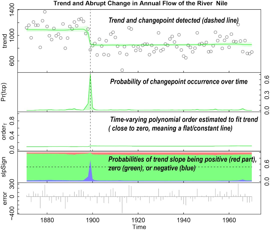
# Apply beast to trend-only data. 'Nile' is the ANNUAL river flow of the river
# Nile at Aswan since 1871. It is a 'ts' object; its time attributes (start=1871,
# end=1970,frequency=1) are used to replace the user-supplied start,deltat, and freq,
# if any.
data(Nile)
plot(Nile)
attributes(Nile) # a ts object with time attributes (i.e., tsp=(start,end,freq)
o = beast(Nile) # start=1871, delta=1, and freq=1 taken from Nile itself
plot(o)
o = beast(Nile, # the same as above. The user-supplied values (i.e., 2023,
start=2023, # 9999) are ignored bcz Nile carries its own time attributes.
period=9999, # Its frequency tag is 1 (i.e., trend-only), so season='none'
season='harmonic' # is used instead of the supplied 'harmonic'
)
#------------------------------------Example 7----------------------------------------#
# NileVec is a pure data vector. The first run below is WRONG bcz NileVec was assumed
# to have a perodic component by default and beast gets a best estimate of freq=6 while
# the true value is freq=1. To fit a trend-only model, season='none' has to be explicitly
# specified, as in the 2nd & 3rd funs.
NileVec = as.vector(Nile) # NileVec is not a ts obj but a pure numeric data vector
o = beast(NileVec) # WRONG WAY to call: No time attributes available to interpret
# NileVec. By default, beast assumes season='harmonic', start=1,
# & deltat=1. 'freq' is missing and guessed to be 6 (WRONG).
plot(o) # WRONG Results: The result has a suprious seasonal component
o=beast(NileVec,season='none') # The correct way to call: Use season='none' for trend-only
# analysis; the default time is the integer indices
# "1:length(NileVec)'.
print(o$time)
o=beast(NileVec, # Recommended way to call: The true time attributes are
start = 1871, # given explicitly through start and deltat (or freq if
deltat = 1, # there is a cyclic/seasonal cmponent).
season = 'none')
print(o$time)
plot(o)
#------------------------------------Example 8----------------------------------------#
# beast can handle missing data. co2 is a monthly time series (i.e.,freq=12) starting
# from Jan 1959. We generate some missing values at random indices
## Not run:
data(co2)
attributes(co2) # A ts object with time attributes (i.e., tsp)
badIdx = sample( 1:length(co2), 50) # Get a set of random indices
co2[badIdx] = NA # Insert some data gaps
out=beast(co2) # co2 is a ts object and its 'tsp' time attributes are used to get the
# true time info. No need to specify 'start','deltat', & freq explicity.
out=beast(co2, # The supplied time/period values will be ignored bcz
start = c(1959,1,15),# co2 is a ts object; the correct period = 1 will be
deltat = 1/12, # used.
period = 365)
print(out)
plot(out)
## End(Not run)
#------------------------------------Example 9----------------------------------------#
# Apply beast to time seris-like sequence data: the unit of sequences is not
# necessarily time.
data(CNAchrom11) # DNA copy number alterations in Chromesome 11 for cell line GM05296
# The data is orderd by genomic position (not time), and the values
# are the log2-based intensity ratio of copy numbers between the sample
# the reference. A value of zero means no gain or loss in copy number.
o = beast(CNAchrom11,season='none') # season is a misnomer here bcz the data has nothing
# to do with time. Regardless, we fit only a trend.
plot(o)
#------------------------------------Example 10---------------------------------------#
# Apply beast to time seris-like data: the unit of sequences is not necessarily time.
# Age of Death of Successive Kings of England
# If the data link is deprecated, install the time series data library instead,
# which is available at https://pkg.yangzhuoranyang.com/tsdl/
# install.packages("devtools")
# devtools::install_github("FinYang/tsdl")
# kings = tsdl::tsdl[[293]]
kings = scan("http://robjhyndman.com/tsdldata/misc/kings.dat",skip=3)
out = beast(kings,season='none')
plot(out)
#------------------------------------Example 11---------------------------------------#
# Another example from the tsdl data library
# Number of monthly births in New York from Jan 1946 to Dec 1959
# If the data link becomes invalid, install the time series data package instead
# install.packages("devtools")
# devtools::install_github("FinYang/tsdl")
# kings = tsdl::tsdl[[534]]
births = scan("http://robjhyndman.com/tsdldata/data/nybirths.dat")
out = beast(births,start=c(1946,1,15), deltat=1/12 )
plot(out) # the result is wrong bcz the guessed freq via auto-correlation by beast
# is 2 rather than 12, so we recommend always specifying 'freq' explicitly
# for those time series with a periodic component, as shown below.
out = beast(births,start=c(1946,1,15), deltat=1/12, freq =12 )
out = beast(births,start=c(1946,1,15), deltat=1/12, period=1.0 )
plot(out)
# Fit the seasonal component using a singular-value-decompostion-based basis functions
# rathat than the default harmonic sin/cos basis functions.
out = beast(births,start=c(1946,1,15), deltat=1/12, period=1.0, season="svd" )
plot(out)
#------------------------------------Example 12---------------------------------------#
# Daily confirmed COVID-19 new cases and deaths across the globe
## Not run:
data(covid19)
plot(covid19$date, covid19$newcases, type='l')
newcases = sqrt( covid19$newcases ) # Apply a square root-transformation
# This ts varies periodically every 7 days. 7 days can't be precisely represented
# in the unit of year bcz some years has 365 days and others has 366. BEAST can hanlde
# this in two ways.
#(1) Use the date number as the time unit--the num of days lapsed since 1970-01-01.
datenum = as.numeric(covid19$date)
o = beast(newcases, start=min(datenum), deltat=1, period=7)
o$time = as.Date(o$time, origin='1970-01-01') # Convert from integers to Date.
plot(o)
#(2) Use strings to explicitly specify deltat and period with a unit.
startdate = covid19$date[1]
o = beast(newcases, start=startdate, deltat='1day', period='7days')
plot(o)
## End(Not run)
#------------------------------------Example 13---------------------------------------#
# The old API interface of beast is still made available but NOT recommended. It is
# kept mainly to ensure the working of the sample code on Page 475 in the text
# Ecological Metods by Drs. Southwood and Henderson.
## Not run:
# The interface as shown here will be deprecated and NOT recommended.
beast(Yellowstone, 24) #24 is the freq: number of datapoints per period
# Specify the model or MCMC parameters through opt as in Rbeast v0.2
opt=list() #Create an empty list to append individual model parameters
opt$period=24 #Period of the cyclic component (i.e.,freq in the new version)
opt$minSeasonOrder=2 #Min harmonic order allowed in fitting season component
opt$maxSeasonOrder=8 #Max harmonic order allowed in fititing season component
opt$minTrendOrder=0 #Min polynomial order allowed to fit trend (0 for constant)
opt$maxTrendOrder=1 #Max polynomial order allowed to fit trend (1 for linear term)
opt$minSepDist_Season=20#Min separation time btw neighboring season changepoints
opt$minSepDist_Trend=20 #Min separation time btw neighboring trend changepoints
opt$maxKnotNum_Season=4 #Max number of season changepoints allowed
opt$maxKnotNum_Trend=10 #Max number of trend changepoints allowed
opt$omittedValue=NA #A customized value to indicate bad/missing values in the time
#series, in additon to those NA or NaN values.
# The following parameters used to configure the reverisible-jump MCMC (RJMCC) sampler
opt$chainNumber=2 #Number of parallel MCMC chains
opt$sample=1000 #Number of samples to be collected per chain
opt$thinningFactor=3 #A factor to thin chains
opt$burnin=500 #Number of burn-in samples discarded at the start
opt$maxMoveStepSize=30 #For the move proposal, the max window allowed in jumping from
#the current changepoint
opt$resamplingSeasonOrderProb=0.2 #The probability of selecting a re-sampling proposal
#(e.g., resample seasonal harmonic order)
opt$resamplingTrendOrderProb=0.2 #The probability of selecting a re-sampling proposal
#(e.g., resample trend polynomial order)
opt$seed=65654 #A seed for the random generator: If seed=0,random numbers differ
#for different BEAST runs. Setting seed to a chosen non-zero integer
#will allow reproducing the same result for different BEAST runs.
beast(Yellowstone, opt)
## End(Not run)
#------------------------------------Example 14---------------------------------------#
# Fit a model with an outlier component: Y = trend + outlier + error.
# Outliers here refer to spikes or dips at isolated points that can't be capatured by the
# trend
## Not run:
NileVec = as.vector(Nile)
NileVec[50] = NileVec[50] + 1500 # Add an large artificial spike at t=50
o = beast(NileVec, season='none', hasOutlier=TRUE)
plot(o)
o = beast(Nile, season='none', hasOutlier=TRUE) # Fit a model with outliers
plot(o)
## End(Not run)
Bayesian decomposition of irregular time series for changepoints, trend, and seasonality
Description
beast.irreg applies the BEAST (Bayesian Estimator of Abrupt change, Seasonal change, and Trend) model to irregular or unordered time series or 1D sequential data. BEAST is a Bayesian model averaging algorithm for decomposing time series or other 1D sequential data into individual components, including abrupt changes, trends, and periodic/seasonal variations. It is useful for changepoint detection (e.g., breakpoints or structural breaks), nonlinear trend analysis, time series decomposition, and time series segmentation. beast123 is a low-level interface to BEAST.
Internally, irregular observations are first aggregated into an evenly spaced (regular) time series at a user-specified time interval, and then decomposed into individual components such as abrupt changes, nonlinear trends, and periodic/seasonal variations.
Usage
  beast.irreg(
       y,
       time,
       deltat         = NULL,
       season         = c("harmonic", "svd", "dummy", "none"),
       period         = NULL,
       scp.minmax     = c(0, 10),   sorder.minmax   = c(0, 5),
       tcp.minmax     = c(0, 10),   torder.minmax   = c(0, 1),
       sseg.min       = NULL,       sseg.leftmargin = NULL,  sseg.rightmargin = NULL,
       tseg.min       = NULL,       tseg.leftmargin = NULL,  tseg.rightmargin = NULL,
       s.complexfct   = 0.0,
       t.complexfct   = 0.0,
       method         = c("bayes", "bic", "aic", "aicc", "hic",
	                      "bic0.25", "bic0.5", "bic1.5", "bic2"),
       detrend        = FALSE,
       deseasonalize  = FALSE,
       mcmc.seed      = 0,
       mcmc.burnin    = 200,
       mcmc.chains    = 3,
       mcmc.thin      = 5,
       mcmc.samples   = 8000,
       precValue      = 1.5,
       precPriorType  = c("componentwise", "uniform", "constant", "orderwise"),
       hasOutlier     = FALSE,
       ocp.minmax     = c(0, 10),
       print.param    = TRUE,
       print.progress = TRUE,
       print.warning  = TRUE,
       quiet          = FALSE,
       dump.ci        = FALSE,
       dump.mcmc      = FALSE,
       gui            = FALSE,
       ...
  )
Arguments
y |
If |
time |
|
deltat |
Numeric or character; the time interval used to aggregate the irregular time series into a regular one. The BEAST model is formulated for regular (evenly spaced) data; therefore
To specify the unit explicitly, supply a character string, for example |
season |
Character (default
|
period |
Numeric or character. The period of the seasonal/periodic component in The period must have units consistent with
If |
scp.minmax |
Integer vector of length 2 ( If If both values are 0, no seasonal changepoints are allowed; a global harmonic (or SVD/dummy) model is used, but the most likely harmonic order is still inferred if |
sorder.minmax |
Integer vector of length 2 ( If |
tcp.minmax |
Integer vector of length 2 ( If If both values are 0, no trend changepoints are allowed; a global polynomial trend is used, but the most likely polynomial order is still inferred if |
torder.minmax |
Integer vector of length 2 ( If |
sseg.min |
Integer (
|
sseg.leftmargin |
Integer (
|
sseg.rightmargin |
Integer (
|
tseg.min |
Integer (
|
tseg.leftmargin |
Integer (
|
tseg.rightmargin |
Integer (
|
s.complexfct |
Numeric (default |
t.complexfct |
Numeric scalar (default |
method |
Character (default
|
detrend |
Logical; if |
deseasonalize |
Logical; if |
mcmc.seed |
Integer ( |
mcmc.chains |
Integer ( |
mcmc.thin |
Integer ( |
mcmc.burnin |
Integer ( |
mcmc.samples |
Integer ( |
precValue |
Numeric ( |
precPriorType |
Character; one of
|
hasOutlier |
Logical; if
Outliers are modeled as changepoints that cannot be captured by trend or seasonal terms. |
ocp.minmax |
Integer vector of length 2 ( |
print.param |
Logical; if |
print.progress |
Logical; if |
print.warning |
Logical; if |
quiet |
Logical; if |
dump.ci |
Logical; if |
dump.mcmc |
Logical; if |
gui |
Logical; if |
... |
Additional implementation-level arguments passed to the underlying |
Value
An object of class "beast", i.e., a list with components similar to those returned by beast and beast123. Below we assume the input y is a single time series of length N:
time |
Numeric vector of length |
data |
A vector, matrix, or 3D array containing a copy of the regularized input data if |
marg_lik |
Numeric; the (average) model marginal likelihood. Larger values correspond to better fits for a given time series (e.g., |
R2 |
Numeric; coefficient of determination ( |
RMSE |
Numeric; root mean squared error of the fitted model. |
sig2 |
Numeric; estimated variance of the model residuals. |
trend |
List containing summaries for the estimated trend component:
|
season |
List containing summaries for the estimated seasonal/periodic component (if present):
|
outlier |
|
Note
The three functions beast(), beast.irreg(), and beast123() implement the same BEAST algorithm but expose different APIs:
-
beast()operates on regular (evenly spaced) time series. -
beast.irreg()accepts irregular/unordered data and internally aggregates it to regular intervals. -
beast123()exposes a low-level interface via four lists:metadata,prior,mcmc, andextra.
There is a one-to-one correspondence between arguments of beast() / beast.irreg() and fields in metadata, prior, mcmc, and extra used by beast123(), Examples include:
start | <-> | metadata$startTime |
deltat | <-> | metadata$deltaTime |
deseasonalize | <-> | metadata$deseasonalize |
hasOutlier | <-> | metadata$hasOutlier |
scp.minmax[1:2] | <-> | prior$seasonMinKnotNum, prior$seasonMaxKnotNum |
sorder.minmax[1:2] | <-> | prior$seasonMinOrder, prior$seasonMaxOrder |
sseg.min | <-> | prior$seasonMinSepDist |
tcp.minmax[1:2] | <-> | prior$trendMinKnotNum, prior$trendMaxKnotNum |
torder.minmax[1:2] | <-> | prior$trendMinOrder, prior$trendMaxOrder |
tseg.leftmargin | <-> | prior$trendLeftMargin |
tseg.rightmargin | <-> | prior$trendRightMargin |
s.complexfct | <-> | prior$seasonComplexityFactor |
t.complexfct | <-> | prior$trendComplexityFactor |
mcmc.seed | <-> | mcmc$seed |
dump.ci | <-> | extra$computeCredible.
|
Advanced users who need full control over all internal options are encouraged to use beast123() directly.
References
Zhao, K., Wulder, M. A., Hu, T., Bright, R., Wu, Q., Qin, H., Li, Y., Toman, E., Mallick, B., Zhang, X. and Brown, M. (2019). Detecting change-point, trend, and seasonality in satellite time series data to track abrupt changes and nonlinear dynamics: A Bayesian ensemble algorithm. Remote Sensing of Environment, 232, 111181. (The main BEAST algorithm paper.)
Zhao, K., Valle, D., Popescu, S., Zhang, X. and Mallick, B. (2013). Hyperspectral remote sensing of plant biochemistry using Bayesian model averaging with variable and band selection. Remote Sensing of Environment, 132, 102–119. (The Bayesian MCMC scheme used in BEAST.)
Hu, T., Toman, E. M., Chen, G., Shao, G., Zhou, Y., Li, Y., Zhao, K. and Feng, Y. (2021). Mapping fine-scale human disturbances in a working landscape with Landsat time series on Google Earth Engine. ISPRS Journal of Photogrammetry and Remote Sensing, 176, 250–261. (Example application of BEAST.)
See Also
beast,
beast123,
minesweeper,
tetris,
geeLandsat
Examples
library(Rbeast)


################################################################################
# Note: The BEAST algorithm is implemented for regular time series.
# \code{beast.irreg} accepts irregular data but internally aggregates it to a
# regular series before applying BEAST. For aggregation, both "time" and
# "deltat" are needed to specify the original timestamps via "time" and the desired
# regular interval via "deltat". If a cyclic component exists, "period" should also
# be provided; otherwise BEAST attempts to guess it via autocorrelation.
################################################################################

# 'ohio' is a data.frame containing an irregular Landsat time series of
# reflectances and NDVI at an Ohio site. It includes multiple alternative
# date formats: year (Y), month (M), day (D), day-of-year (doy), R "Date"
# (rdate), and fractional year (time).

data(ohio)
str(ohio)
plot(ohio$rdate, ohio$ndvi, type = "o")  # NDVI is irregular and unordered in time

################################################################################
# Example 1: 'time' as numeric values
# Below, 'time' is given as numeric values, which can be of any arbitray unit. Although
# here 1/12 can be interepreted as 1/12 year, BEAST itself doesn't care about the unit.
# So, the unit of 1/12 is irrelevant for BEAST. 'period' is missing
# and a guess of it is used.
################################################################################

o <- beast.irreg(ohio$ndvi, time = ohio$time, deltat = 1/12)
plot(o)
print(o)

################################################################################
# Example 2: Aggregate to a monthly interval (deltat = 1/12) and provide 'period'
################################################################################

o <- beast.irreg(ohio$ndvi, time = ohio$time, deltat = 1/12, period = 1.0)
# Alternative (deprecated argument 'freq'):
# o <- beast.irreg(ohio$ndvi, time = ohio$time, deltat = 1/12, freq = 12)


## Not run:

################################################################################
# Example 3: Aggregate at a half-monthly interval.
# Here period = 1: freq = period/deltat = 1/(1/24)=24 data points per period
################################################################################

o <- beast.irreg(ohio$ndvi, time = ohio$time, deltat = 1/24, period = 1)

################################################################################
# Example 4: 'time' as  R Dates (i.e, ohio$rdate). Unit is YEAR; 1/12 is ~1 month.
################################################################################

o <- beast.irreg(ohio$ndvi, time = ohio$rdate, deltat = 1/12)

################################################################################
# Example 5: 'time' as date strings. The unit is YEAR such that 1/12 is a month
################################################################################

o=beast.irreg(ohio$ndvi, time=ohio$datestr1,deltat=1/12) #"LT4-1984-03-27"  (YYYY-MM-DD)
o=beast.irreg(ohio$ndvi, time=ohio$datestr2,deltat=1/12) #"LT4-1984087ndvi" (YYYYDOY)
o=beast.irreg(ohio$ndvi, time=ohio$datestr3,deltat=1/12) #"1984,, 3/ 27"    (YYYY M D)

################################################################################
# Example 6: 'time' as date strings with explicit format specifiers
################################################################################

TIME <- list()
TIME$datestr <- ohio$datestr1
TIME$strfmt  <- "LT4-YYYY-MM-DD"    # e.g., "LT4-1984-03-27"
o <- beast.irreg(ohio$ndvi, time = TIME, deltat = 1/12)

TIME <- list()
TIME$datestr <- ohio$datestr2
TIME$strfmt  <- "LT4-YYYYDOYndvi"   # e.g., "LT4-1984087ndvi"
o <- beast.irreg(ohio$ndvi, time = TIME, deltat = 1/12)

################################################################################
# Example 7: 'time' as a list of date components
################################################################################

TIME <- list()
TIME$year  <- ohio$Y
TIME$month <- ohio$M
TIME$day   <- ohio$D
o <- beast.irreg(ohio$ndvi, time = TIME, deltat = 1/12)

TIME <- list()
TIME$year <- ohio$Y
TIME$doy  <- ohio$doy
o <- beast.irreg(ohio$ndvi, time = TIME, deltat = 1/12)


## End(Not run)
Bayesian time series decomposition into changepoints, trend, and seasonal/periodic components
Description
BEAST is a Bayesian model averaging algorithm for decomposing time series or other 1D sequential data into individual components, including abrupt changes, trends, and periodic/seasonal variations. It is useful for changepoint detection (e.g., breakpoints or structural breaks), nonlinear trend analysis, time series decomposition, and time series segmentation. beast123 is a low-level interface to BEAST.
Usage
beast123(
  Y,
  metadata = list(),
  prior    = list(),
  mcmc     = list(),
  extra    = list(),
  season   = c("harmonic","svd","dummy","none"),
  method   = c("bayes","bic","aic","aicc","hic",
               "bic0.25","bic0.5","bic1.5","bic2"),
  ...
)
Arguments
Y |
|
metadata |
If missing, default values are used. However, when When
|
prior |
|
mcmc |
|
extra |
|
season |
Character (default
|
method |
Character (default
|
... |
Additional parameters reserved for future extensions; currently unused. |
Value
The output is a list object of class "beast" containing the following fields. Exact dimensions depend on the input Y and extra$whichOutputDimIsTime. The descriptions below assume a single time series input of length N; for 2D/3D inputs, interpret the results according to the 2D/3D dimensions.
time |
A numeric vector of length |
data |
A vector, matrix, or 3D array; a copy of the input |
marg_lik |
Numeric; the average marginal likelihood of the sampled models. Larger values indicate better fit for a given time series. |
R2 |
Numeric; coefficient of determination (R-squared) of the fitted model. |
RMSE |
Numeric; root mean squared error of the fitted model. |
sig2 |
Numeric; estimated variance of the residual error. |
trend |
|
season |
|
outlier |
|
References
Zhao, K., Wulder, M.A., Hu, T., Bright, R., Wu, Q., Qin, H., Li, Y., Toman, E., Mallick, B., Zhang, X. and Brown, M., 2019. Detecting change-point, trend, and seasonality in satellite time series data to track abrupt changes and nonlinear dynamics: A Bayesian ensemble algorithm. Remote Sensing of Environment, 232, p.111181 (the beast algorithm paper).
Zhao, K., Valle, D., Popescu, S., Zhang, X. and Mallick, B., 2013. Hyperspectral remote sensing of plant biochemistry using Bayesian model averaging with variable and band selection. Remote Sensing of Environment, 132, pp.102-119 (the Bayesian MCMC scheme used in beast).
Hu, T., Toman, E.M., Chen, G., Shao, G., Zhou, Y., Li, Y., Zhao, K. and Feng, Y., 2021. Mapping fine-scale human disturbances in a working landscape with Landsat time series on Google Earth Engine. ISPRS Journal of Photogrammetry and Remote Sensing, 176, pp.250-261(a beast application paper).
See Also
beast,
beast.irreg,
minesweeper,
tetris,
geeLandsat
Examples
#-------------------------------- NOTE ----------------------------------------------#
# beast123() is an all-inclusive function that unifies the functionality of beast()
# and beast.irreg(). It can handle single, multiple, or 3D stacked time series, either
# regular or irregular. It allows customization via four list arguments:
#   metadata -- additional information about the input Y
#   prior    -- prior parameters for the BEAST model
#   mcmc     -- MCMC settings
#   extra    -- miscellaneous options controlling output and parallel computation
#
# Although functionally similar to beast() and beast.irreg(), beast123() is designed
# to efficiently handle multiple time series concurrently (e.g., stacked satellite
# images) via internal multithreading. When processing stacks of raster layers,
# DO NOT iterate pixel-by-pixel using beast() or beast.irreg() wrapped by external
# parallel tools (e.g., doParallel, foreach). Instead, use beast123(), which
# implements parallelism internally.

#------------------------------ Example 1: seasonal time series ----------------------#
# Yellowstone is a half-monthly NDVI time series of length 774 for a site in Yellowstone
# starting from July 1-15, 1981 (start ~ c(1981, 7, 7); 24 observations per year).

library(Rbeast)
data(Yellowstone)
plot(Yellowstone)

# Below, the four optional arguments are omitted, so default values are used.
# By default, Y is assumed to be regular with a seasonal component. The actual
# default values are printed at the start of the run and can be used as templates
# for customization.

  o <- beast123(Yellowstone)
  plot(o)


#------------------------------ Example 2: trend-only series -------------------------#
# Nile is an annual river flow time series (no periodic variation). Set season = "none"
# to indicate trend-only analysis. Default values are used for other options.
# Unlike beast(), beast123() does NOT use the time attributes of a 'ts' object.
# For example, Nile is treated as numeric data only with the default times
# 1:length(Nile); its (start=1871, end=1970, freq=1) attributes are ignored
# unless specified through 'metadata'.


  o <- beast123(Nile, season = "none")
  o <- beast123(Nile, extra = list(dumpInputData = TRUE, quiet = TRUE),
                season = "none")
  o <- beast123(Nile, metadata = list(startTime = 1871, hasOutlier = TRUE),
                season = "none")
  plot(o)


#------------------------------ Example 3: full API usage ---------------------------#
# Explicitly specify metadata, prior, mcmc, and extra. Among these, 'prior' contains
# the true statistical model parameters; the others configure input, output, and
# computation.

## Not run:

  # metadata: extra information describing the input time series Y.
  metadata <- list()
  # metadata$isRegularOrdered <- TRUE    # no longer used in this version
  metadata$whichDimIsTime      <- 1      # which dimension is time for 2D/3D inputs
  metadata$startTime           <- c(1981, 7, 7)
  # alternatively: metadata$startTime <- 1981.5137
  #                metadata$startTime <- as.Date("1981-07-07")
  metadata$deltaTime           <- 1/24   # half-monthly: 24 obs/year
  metadata$period              <- 1.0    # 1-year period: 24 * (1/24) = 1
  metadata$omissionValue       <- NaN    # NaNs are omitted by default
  metadata$maxMissingRateAllowed <- 0.75 # skip series with > 75
  metadata$deseasonalize       <- FALSE  # do not pre-remove global seasonality
  metadata$detrend             <- FALSE  # do not pre-remove global trend

  # prior: only true model parameters specifying the Bayesian formulation
  prior <- list()
  prior$seasonMinOrder    <- 1     # min harmonic order allowed to fit seasonal cmpnt
  prior$seasonMaxOrder    <- 5     # max harmonic order allowed to fit seasonal cmpnt
  prior$seasonMinKnotNum  <- 0     # min number of changepnts in seasonal cmpnt
  prior$seasonMaxKnotNum  <- 3     # max number of changepnts in seasonal cmpnt
  prior$seasonMinSepDist  <- 10    # min inter-chngpts separation for seasonal cmpnt
  prior$trendMinOrder     <- 0     # min polynomial order allowed to fit trend cmpnt
  prior$trendMaxOrder     <- 1     # max polynomial order allowed to fit trend cmpnt
  prior$trendMinKnotNum   <- 0     # min number of changepnts in trend cmpnt
  prior$trendMaxKnotNum   <- 15    # max number of changepnts in trend cmpnt
  prior$trendMinSepDist   <- 5     # min inter-chngpts separation for trend cmpnt
  prior$precValue         <- 10.0  # Initial value of precision parameter(no need
                                   # to change it unless for precPrioType='const')
  prior$precPriorType     <- "uniform"  # "constant", "uniform", "componentwise", "orderwise"

  # mcmc: settings for the MCMC sampler
  mcmc <- list()
  mcmc$seed                      <- 9543434  # arbitray seed for random number generator
  mcmc$samples                   <- 3000     # samples collected per chain
  mcmc$thinningFactor            <- 3        # take every 3rd sample and discard others
  mcmc$burnin                    <- 150      # discard the initial 150 samples per chain
  mcmc$chainNumber               <- 3        # number of chains
  mcmc$maxMoveStepSize           <- 4        # max random jump step when proposing new chngpts
  mcmc$trendResamplingOrderProb  <- 0.10     # prob of choosing to resample polynomial order
  mcmc$seasonResamplingOrderProb <- 0.10     # prob of choosing to resample harmonic order
  mcmc$credIntervalAlphaLevel    <- 0.95     # the significance level for credible interval

  # extra: output and computation options
  extra <- list()
  extra$dumpInputData         <- FALSE  # If true, a copy of input time series is outputted
  extra$whichOutputDimIsTime  <- 1      # For 2D or 3D inputs, which dim of the output refers
                                        # to time? Ignored if the input is a single time series
  extra$computeCredible       <- FALSE  # If true, compute CI: computing CI is time-intensive.
  extra$fastCIComputation     <- TRUE   # If true, a faster way is used to get CI, but it is
                                        # still time-intensive. That is why the function beast()
                                        # is slow because it always compute CI.
  extra$computeSeasonOrder    <- FALSE  # If true, dump the estimated harmonic order over time
  extra$computeTrendOrder     <- FALSE  # If true, dump the estimated polynomial order over time
  extra$computeSeasonChngpt   <- TRUE   # If true, get the most likely locations of s chgnpts
  extra$computeTrendChngpt    <- TRUE   # If true, get the most likely locations of t chgnpts
  extra$computeSeasonAmp      <- FALSE  # If true, get time-varying amplitude of seasonality
  extra$computeTrendSlope     <- FALSE  # If true, get time-varying slope of trend
  extra$tallyPosNegSeasonJump <- FALSE  # If true, get those changpts with +/- jumps in season
  extra$tallyPosNegTrendJump  <- FALSE  # If true, get those changpts with +/- jumps in trend
  extra$tallyIncDecTrendJump  <- FALSE  # If true, get those changpts with increasing/
                                        # decreasing trend slopes
  extra$printProgress         <- TRUE
  extra$printParameter        <- TRUE
  extra$quiet                 <- FALSE  # if TRUE, print warning messages, if any
  extra$consoleWidth          <- 0      # If 0, the console width is from the current console
  extra$numThreadsPerCPU      <- 2      # 'numThreadsPerCPU' and 'numParThreads' are used to
  extra$numParThreads         <- 0      #   configure multithreading runs; they're used only
                                        #   if Y has multiple time series (e.g.,stacked images)

  o <- beast123(Yellowstone, metadata, prior, mcmc, extra, season = "harmonic")
  plot(o)

## End(Not run)

#------------------------------ Example 4: irregular time series ---------------------#
# ohio is a data frame of Landsat NDVI observations at unevenly spaced times.


## Not run:

  data(ohio)
  str(ohio)

  ###################################################################################
  # Individual times are provided as fractional years via ohio$time

  metadata <- list()
  metadata$time      <- ohio$time  # Must supply individual times for irregular inputs
  metadata$deltaTime <- 1/12       # Must supply the desired time interval for aggregation
  metadata$period    <- 1.0
  o <- beast123(ohio$ndvi, metadata)   # defaults used for missing parameters

  ###################################################################################
  # Another accepted time format: Ohio dates as Date objects
  class(ohio$rdate)

  metadata <- list()
  metadata$time      <- ohio$rdate # Must supply individual times for irregular inputs
  metadata$deltaTime <- 1/12       # Must supply the desired time interval for aggregation
  o <- beast123(ohio$ndvi, metadata)  # Default values used for those missing parameters

  ###################################################################################
  # Another accepted time format: separate Y, M, D columns
  ohio$Y      # Year
  ohio$M      # Month
  ohio$D      # Day

  metadata <- list()
  metadata$time$year   <- ohio$Y   # Must supply individual times for irregular inputs
  metadata$time$month  <- ohio$M
  metadata$time$day    <- ohio$D
  metadata$deltaTime   <- 1/12     # Must supply the desired time interval for aggregation
  o <- beast123(ohio$ndvi, metadata) # Default values used for those missing parameters

  ###################################################################################
  # Another accepted time format: year and DOY
  ohio$Y        # Year
  ohio$doy      # Day of year

  metadata <- list()
  metadata$time$year  <- ohio$Y   # Must supply individual times for irregular inputs
  metadata$time$doy   <- ohio$doy
  metadata$deltaTime  <- 1/12     # Must supply the desired time interval for aggregation
  o <- beast123(ohio$ndvi, metadata) # Default values used for those missing parameters


  ###################################################################################
  # Another accepted time format: date strings with custom strfmt
  ohio$datestr1

  metadata <- list()
  metadata$time$datestr  <- ohio$datestr1
  metadata$time$strfmt   <- "????yyyy?mm?dd"
  metadata$deltaTime     <- 1/12
  o <- beast123(ohio$ndvi, metadata)

 ###################################################################################
 # Another accepted time format: date strings with custom strfmt
  ohio$datestr2

  metadata <- list()
  metadata$deltaTime     <- 1/12
  metadata$time$datestr  <- ohio$datestr2
  metadata$time$strfmt   <- "????yyyydoy????"
  o <- beast123(ohio$ndvi, metadata)

 ###################################################################################
 # Another accepted time format: date strings with custom strfmt
  ohio$datestr3

  metadata <- list()
  metadata$deltaTime     <- 1/12
  metadata$time$datestr  <- ohio$datestr3
  metadata$time$strfmt   <- "Y,,M/D"
  o <- beast123(ohio$ndvi, metadata)

## End(Not run)


#------------------ Example 5: multiple time series (matrix input) -------------------#
# simdata is a 2D matrix of dimension 300 x 3, representing 3 time series of length 300.

## Not run:
  data(simdata)  # dim of simdata: 300 x 3 (time x num_of_time_series)
  dim(simdata)   # the first dimenion refer to time (i.e, 300)

  metadata <- list()
  metadata$whichDimIsTime <- 1  # first dimension is time
  metadata$period         <- 24 # assume startTime = 1, deltaTime = 1 by default

  extra <- list()
  extra$whichOutputDimIsTime <- 2  # Which dim of the output arrays refers to  time?

  o <- beast123(simdata, metadata, extra = extra)

  # Lists of inputs args can also be provided inline:
  o <- beast123(simdata,
                metadata = list(whichDimIsTime = 1, period = 24),
                extra    = list(whichOutputDimIsTime = 2))

  # Field names can be shortened, provided no ambiguity arises:
  o <- beast123(simdata,
                metadata = list(whichDim = 1, per = 24),
                extra    = list(whichOut = 2))

  #------------------ Example 5b: transposed simdata ---------------------------------#
  simdata1 <- t(simdata)   # 3 (series) x 300 (time)
                           # dim of simdata1: 3 x 300 (num of ts  x time )

  metadata <- list()
  metadata$whichDimIsTime <- 2  # time is second dimension
  metadata$period         <- 24 # assume startTime = 1, deltaTime = 1 by default
  o <- beast123(simdata1, metadata)

  o <- beast123(simdata1, metadata = list(whichDim = 2, per = 24))

## End(Not run)

#------------------ Example 6: 3D stacked image time series -------------------------#
# imagestack$ndvi is a 3D array of size 12 x 9 x 1066 (row x col x time). Each pixel
# corresponds to a time series of length 1066.

## Not run:
  data(imagestack)
  dim(imagestack$ndvi)   # 12 x 9 x 1066
  imagestack$datestr     # A character vector of 1066 date strings

  metadata <- list()
  metadata$whichDimIsTime <- 3  # Which dim of the input refer to time for 3D inputs?
                                # 1066 is the ts length, so dim is set to '3' here.
                                # In this example, this arg is not needed because
                                # the time$datestr can also help to match and pick up
                                # the right time dimesion of imagestack$ndvi.
  metadata$time$datestr   <- imagestack$datestr
  metadata$time$strfmt    <- "LT05_018032_20080311.yyyy-mm-dd"
  metadata$deltaTime      <- 1/12   # aggregate to monthly (i.e., 1/12 yr)
  metadata$period         <- 1.0    # 1-year period

  extra <- list()
  extra$dumpInputData    <- TRUE   # Dump a copy of aggregated input ts
  extra$numThreadsPerCPU <- 2      # Each cpu core will be assigned 2 threads
  extra$numParThreads    <- 0      # If 0, total_num_threads=numThreadsPerCPU*num_of_cpu_core
                                   # if >0, used to specify the total number of threads

  # Default values for missing parameters
  o <- beast123(imagestack$ndvi, metadata = metadata, extra = extra)

  print(o, c(5, 3))     # result for pixel at row 5, col 3
  plot(o,  c(5, 3))     # plot result for pixel at row 5, col 3
  image(o$trend$ncp)    # map number of trend changepoints over space

## End(Not run)

#------------------ Example 7: GeoTIFF stacks via raster package --------------------#
# Handle 3D stacked images from a series of NDVI GeoTIFF files (e.g., ndvi.zip with
# 437 NDVI TIFF files of dimension 12 x 9). Example code is available at:
#   https://github.com/zhaokg/Rbeast/blob/master/R/beast123_raster_example.txt
Daily confirmed COVID19 cases and deaths in the world
Description
covid19 is a data frame consisting of daily confirmed COVID19 cases and deaths in the world from Jan 22, 2020 to Dec 16, 2021.
Usage
data(covid19)
Source
https://ourworldindata.org/grapher/daily-covid-cases-deaths?country=~OWID_WRL (last accessed on Dec 16, 2021)
References
Zhao, K., Wulder, M.A., Hu, T., Bright, R., Wu, Q., Qin, H., Li, Y., Toman, E., Mallick, B., Zhang, X. and Brown, M., 2019. Detecting change-point, trend, and seasonality in satellite time series data to track abrupt changes and nonlinear dynamics: A Bayesian ensemble algorithm. Remote Sensing of Environment, 232, p.111181 (the beast algorithm paper).
Zhao, K., Valle, D., Popescu, S., Zhang, X. and Mallick, B., 2013. Hyperspectral remote sensing of plant biochemistry using Bayesian model averaging with variable and band selection. Remote Sensing of Environment, 132, pp.102-119 (the Bayesian MCMC scheme used in beast).
Hu, T., Toman, E.M., Chen, G., Shao, G., Zhou, Y., Li, Y., Zhao, K. and Feng, Y., 2021. Mapping fine-scale human disturbances in a working landscape with Landsat time series on Google Earth Engine. ISPRS Journal of Photogrammetry and Remote Sensing, 176, pp.250-261(a beast application paper).
Examples
 library(Rbeast)
 data(covid19)
 plot(covid19$date, covid19$newcases, type='l')

 ## Not run:

 # Apply a square root-transformation
 newcases = sqrt( covid19$newcases )

 # This time series varies periodically every 7 days. 7 days can't be precisely
 # represented in the unit of year bcz some years has 365 days and others has 366.
 # BEAST can hanlde this in two ways.


 #(1) Use the date number as the time unit--the num of days lapsed since 1970-01-01.

  datenum  = as.numeric(covid19$date)
  o        = beast(newcases, start=min(datenum), deltat=1, period=7)
  o$time   = as.Date(o$time, origin='1970-01-01') # Convert from integers to Date.
  plot(o)

 #(2) Use strings to explicitly specify deltat and period with a unit.

  startdate = covid19$date[1]
  o         = beast(newcases, start=startdate, deltat='1day', period='7days')
  plot(o)


## End(Not run)
Landsat reflectance and NDVI time series from Google Earth Engine
Description
Get Landsat reflectance and NDVI time series from Google Earth Engine given longitude and latitude
Usage
geeLandsat(lon=NA, lat=NA, radius=100, stat='mean',timeout=700)
Arguments
lon |
numeric within [-180,180] |
lat |
numeric within [-90, 90] |
radius |
a positive number ( <=500 meters ); the radius of a buffer around the given latitude and longitude for aggregation. If |
stat |
character; if |
timeout |
integer; the seconds elapsed to wait for connection timeout. See the note for an explanation. |
Value
a data.frame object consisting of dates, sensor type, reflectances, and NDVI for the requested location. It contains only valid and clear-sky values as obtained by referring to the standard clouds flags.
Note
As a poor man's scheme to interact with Google Earth Engine, geeLandsat should be used only for occasional retrieval of Landsat time series at a few sites, NOT for batch downloading for thousands of sites in a R loop. This procedure is provided to get example time series for testing BEAST. Behind the scene, this function calls to a free Python-based server using my own GEE credential. Normally it takes several seconds to retrieve one time series, but as a free cloud service, the Python server only offers 100 seconds of free CPU time per day, with throttling applied. So it may take up to a few mins to get a time series on your end. It may fail due to connection timeout; if so, give it a few tries. If you need to retrieve data for thousands or millions of sites, please contact the author.
References
Zhao, K., Wulder, M.A., Hu, T., Bright, R., Wu, Q., Qin, H., Li, Y., Toman, E., Mallick, B., Zhang, X. and Brown, M., 2019. Detecting change-point, trend, and seasonality in satellite time series data to track abrupt changes and nonlinear dynamics: A Bayesian ensemble algorithm. Remote Sensing of Environment, 232, p.111181 (the beast algorithm paper).
Zhao, K., Valle, D., Popescu, S., Zhang, X. and Mallick, B., 2013. Hyperspectral remote sensing of plant biochemistry using Bayesian model averaging with variable and band selection. Remote Sensing of Environment, 132, pp.102-119 (the Bayesian MCMC scheme used in beast).
Hu, T., Toman, E.M., Chen, G., Shao, G., Zhou, Y., Li, Y., Zhao, K. and Feng, Y., 2021. Mapping fine-scale human disturbances in a working landscape with Landsat time series on Google Earth Engine. ISPRS Journal of Photogrammetry and Remote Sensing, 176, pp.250-261(a beast application paper).
See Also
beast, beast.irreg, beast123, minesweeper, tetris
Examples
 library(Rbeast)
## Not run:
 df = geeLandsat(lon=-80.983877,lat= 40.476882) #if it fails, try a few more times before giving up
 print(df)

## End(Not run)
A monthly Google Trend time series of the US search interest in the word "beach"
Description
googletrend_beach is a ts object comprising monthly search interest in "beach" from the United States, as reported from Google Trends. Sudden changes in the search trend are attributed to extreme weather events or the covid19 outbreak
Usage
data(googletrend_beach)
Source
https://trends.google.com/trends/explore?date=all&geo=US&q=beach
References
Zhao, K., Wulder, M.A., Hu, T., Bright, R., Wu, Q., Qin, H., Li, Y., Toman, E., Mallick, B., Zhang, X. and Brown, M., 2019. Detecting change-point, trend, and seasonality in satellite time series data to track abrupt changes and nonlinear dynamics: A Bayesian ensemble algorithm. Remote Sensing of Environment, 232, p.111181 (the beast algorithm paper).
Zhao, K., Valle, D., Popescu, S., Zhang, X. and Mallick, B., 2013. Hyperspectral remote sensing of plant biochemistry using Bayesian model averaging with variable and band selection. Remote Sensing of Environment, 132, pp.102-119 (the Bayesian MCMC scheme used in beast).
Hu, T., Toman, E.M., Chen, G., Shao, G., Zhou, Y., Li, Y., Zhao, K. and Feng, Y., 2021. Mapping fine-scale human disturbances in a working landscape with Landsat time series on Google Earth Engine. ISPRS Journal of Photogrammetry and Remote Sensing, 176, pp.250-261(a beast application paper).
Examples
 library(Rbeast)
 data(googletrend_beach) # A monthly ts starting from Jan 2004

 o = beast(googletrend_beach )
 plot(o)
Decades of Landsat NDVI time series over a small area in Ohio
Description
imagestack is a LIST containing Landsat-derived NDVI image chips at an Ohio site
Usage
data(imagestack)
Source
Landsat images courtesy of the U.S. Geological Survey
References
Zhao, K., Wulder, M.A., Hu, T., Bright, R., Wu, Q., Qin, H., Li, Y., Toman, E., Mallick, B., Zhang, X. and Brown, M., 2019. Detecting change-point, trend, and seasonality in satellite time series data to track abrupt changes and nonlinear dynamics: A Bayesian ensemble algorithm. Remote Sensing of Environment, 232, p.111181 (the beast algorithm paper).
Zhao, K., Valle, D., Popescu, S., Zhang, X. and Mallick, B., 2013. Hyperspectral remote sensing of plant biochemistry using Bayesian model averaging with variable and band selection. Remote Sensing of Environment, 132, pp.102-119 (the Bayesian MCMC scheme used in beast).
Hu, T., Toman, E.M., Chen, G., Shao, G., Zhou, Y., Li, Y., Zhao, K. and Feng, Y., 2021. Mapping fine-scale human disturbances in a working landscape with Landsat time series on Google Earth Engine. ISPRS Journal of Photogrammetry and Remote Sensing, 176, pp.250-261(a beast application paper).
Examples
 data(imagestack)
 imagestack$datestr # A string vector containg the observation dates of individual ndvi images
 ## Not run:
 imagestack$ndvi    # NDVI images collected over the past several deccades

## End(Not run)
 plot(imagestack$ndvi[3,4,],type='l') # Plot the raw data at a pixel
The Minesweeper game in R
Description
A poor man's implementation of the minesweeper game in R. Yes, you are right: it has nothing to do with time series decomposition, changepoint detection, and time series segmentation. Its only remote connection to Rbeast is that this is a practice script I wrote to learn R graphics for implementing Rbeast.

Usage
minesweeper(height=15, width=12, prob=0.1)
Arguments
height |
integer; number of rows of the mine grid along the vertical direction. |
width |
integer; number of columns of the mine grid along the horizontal direction. |
prob |
numeric; a fraction between 0 and 1 to specify the probability of mine occurrence in the mine grid. |
Value
Instructions:
LEFT-click to clear a spot.
RIGHT-click to flag a spot.
MIDDLE-click(wheel) a cleared and numbered spot to open neighbor spots, if flagged correctly.
Click Restart for a new game
Note
An interactive graphics window is needed to run this function correctly. So it won't run in RStudio's plot pane. The function will use the x11() or x11(type='Xlib') graphic device to open a pop-up window.
References
Zhao, K., Wulder, M.A., Hu, T., Bright, R., Wu, Q., Qin, H., Li, Y., Toman, E., Mallick, B., Zhang, X. and Brown, M., 2019. Detecting change-point, trend, and seasonality in satellite time series data to track abrupt changes and nonlinear dynamics: A Bayesian ensemble algorithm. Remote Sensing of Environment, 232, p.111181 (the beast algorithm paper).
Zhao, K., Valle, D., Popescu, S., Zhang, X. and Mallick, B., 2013. Hyperspectral remote sensing of plant biochemistry using Bayesian model averaging with variable and band selection. Remote Sensing of Environment, 132, pp.102-119 (the Bayesian MCMC scheme used in beast).
Hu, T., Toman, E.M., Chen, G., Shao, G., Zhou, Y., Li, Y., Zhao, K. and Feng, Y., 2021. Mapping fine-scale human disturbances in a working landscape with Landsat time series on Google Earth Engine. ISPRS Journal of Photogrammetry and Remote Sensing, 176, pp.250-261(a beast application paper).
See Also
beast, beast.irreg, beast123, tetris, geeLandsat
Examples
 library(Rbeast)

 ## Not run:
 minesweeper()

 # A mine field of size 20x25 with rougly a 15
 minesweeper(20,25,0.15)

## End(Not run)
An irregular Landsat NDVI time series at an Ohio site
Description
ohio is a data.frame object comprising decades of Landsat-observed surface reflectances and NDVI at an Ohio site
Usage
data(ohio)
Source
Landsat images courtesy of the U.S. Geological Survey
References
Zhao, K., Wulder, M.A., Hu, T., Bright, R., Wu, Q., Qin, H., Li, Y., Toman, E., Mallick, B., Zhang, X. and Brown, M., 2019. Detecting change-point, trend, and seasonality in satellite time series data to track abrupt changes and nonlinear dynamics: A Bayesian ensemble algorithm. Remote Sensing of Environment, 232, p.111181 (the beast algorithm paper).
Zhao, K., Valle, D., Popescu, S., Zhang, X. and Mallick, B., 2013. Hyperspectral remote sensing of plant biochemistry using Bayesian model averaging with variable and band selection. Remote Sensing of Environment, 132, pp.102-119 (the Bayesian MCMC scheme used in beast).
Hu, T., Toman, E.M., Chen, G., Shao, G., Zhou, Y., Li, Y., Zhao, K. and Feng, Y., 2021. Mapping fine-scale human disturbances in a working landscape with Landsat time series on Google Earth Engine. ISPRS Journal of Photogrammetry and Remote Sensing, 176, pp.250-261(a beast application paper).
Examples
 library(Rbeast)
 data(ohio) # Landsat surface references and NDVI at a single pixel observed over time
 str(ohio)

## Not run:
 # ohio$ndvi is a single irregular time series
 y = ohio$ndvi
 o = beast.irreg(y, time=ohio$time,deltat=1/12)
 plot(o)
 print(o)

 # ohio also contains irregular time series of individual spectral bands
 # Below, run the multivariate version of the BEAST algorithm to decompose
 # the 5 time series and detect common changepoints altogether

 y = list(ohio$blue, ohio$green, ohio$red, ohio$nir, ohio$swir1);
 o = beast.irreg(y, time=ohio$time,deltat=1/12, freq=12)
 plot(o)
 print(o)

## End(Not run)
Bayesian changepoint detection and time series decomposition
Description
Plot the result obtained from the beast function.
Usage
## S3 method for class 'beast'
plot(
     x,
     index = 1,
     vars  = c('y','s','scp','sorder','t','tcp','torder','slpsgn','o','ocp','error'),
     col         = NULL,
     main        = "BEAST decomposition and changepoint detection",
     xlab        = 'Time',
     ylab        = NULL,
     cex.main    = 1,
     cex.lab     = 1,
     relative.heights = NULL,
     interactive = FALSE,
     ncpStat     = c('median','mode','mean','pct90','max'),
     ...
   )
Arguments
x |
a "beast" object returned by |
index |
an integer (default to 1 ) or a vector of two integers to specify the index of the time series to plot if |
vars |
a vector of strings indicating the elements or variables of |
relative.heights |
a numeric vector of the same length as that of |
col |
a string vector of the same length as that of |
main |
a string; the main title. |
xlab |
a string: the x axis title. |
ylab |
a string vector of the same length as that of |
cex.main |
cex for the main title |
cex.lab |
cex for the axis title |
interactive |
a bool scalar. If TRUE, an interactive GUI is used for examining individual elements of |
ncpStat |
character. A string to specify which statistic is used for the Number of ChangePoint (ncp). Five values are possible: 'mean', 'mode', 'median','pct90', and 'max'; the default is 'median'. Individual models sampled by BEAST has a varying dimension (e.g., number of changepoints or knots). For example, if mcmc$samples=10, the numbers of changepoints for the 10 sampled models are assumed to be c(0, 2, 4, 1, 1, 2, 7, 6, 6, 1). The mean ncp will be 3.1 (rounded to 3), the median is 2.5 (2), the mode is 1, and the maximum is 7. The 'max' option plots all the changepoints recorded in |
... |
additional parameters to be implemented. |
Value
This function creates various plots to demonstrate the results of a beast decomposition. .
References
Zhao, K., Wulder, M.A., Hu, T., Bright, R., Wu, Q., Qin, H., Li, Y., Toman, E., Mallick, B., Zhang, X. and Brown, M., 2019. Detecting change-point, trend, and seasonality in satellite time series data to track abrupt changes and nonlinear dynamics: A Bayesian ensemble algorithm. Remote Sensing of Environment, 232, p.111181 (the beast algorithm paper).
Zhao, K., Valle, D., Popescu, S., Zhang, X. and Mallick, B., 2013. Hyperspectral remote sensing of plant biochemistry using Bayesian model averaging with variable and band selection. Remote Sensing of Environment, 132, pp.102-119 (the Bayesian MCMC scheme used in beast).
Hu, T., Toman, E.M., Chen, G., Shao, G., Zhou, Y., Li, Y., Zhao, K. and Feng, Y., 2021. Mapping fine-scale human disturbances in a working landscape with Landsat time series on Google Earth Engine. ISPRS Journal of Photogrammetry and Remote Sensing, 176, pp.250-261(a beast application paper).
See Also
beast, beast.irreg, beast123, plot.beast,minesweeper, tetris, geeLandsat
Examples
 library(Rbeast)
 data(simdata)
## Not run:
 result=beast123(simdata, metadata=list(whichDimIsTime=1))
 plot(result,1)
 plot(result,2)

## End(Not run)
Bayesian changepoint detection and time series decomposition
Description
Summarize and print the results obtained from the BEAST time series decomposition and segmentation.
Usage
## S3 method for class 'beast'
print(
     x,
     index = 1,
     ...
	 )
Arguments
x |
a "beast" object returned by |
index |
an integer (default to 1 ) or a vector of two integers to specify the index of the time series to print if |
... |
additional parameters to be implemented. |
Value
Print a summary of changepoints detected for the seasonal or trend component.
References
Zhao, K., Wulder, M.A., Hu, T., Bright, R., Wu, Q., Qin, H., Li, Y., Toman, E., Mallick, B., Zhang, X. and Brown, M., 2019. Detecting change-point, trend, and seasonality in satellite time series data to track abrupt changes and nonlinear dynamics: A Bayesian ensemble algorithm. Remote Sensing of Environment, 232, p.111181 (the beast algorithm paper).
Zhao, K., Valle, D., Popescu, S., Zhang, X. and Mallick, B., 2013. Hyperspectral remote sensing of plant biochemistry using Bayesian model averaging with variable and band selection. Remote Sensing of Environment, 132, pp.102-119 (the Bayesian MCMC scheme used in beast).
Hu, T., Toman, E.M., Chen, G., Shao, G., Zhou, Y., Li, Y., Zhao, K. and Feng, Y., 2021. Mapping fine-scale human disturbances in a working landscape with Landsat time series on Google Earth Engine. ISPRS Journal of Photogrammetry and Remote Sensing, 176, pp.250-261(a beast application paper).
See Also
beast, beast.irreg, beast123, minesweeper, tetris, geeLandsat
Examples
 library(Rbeast)
 data(simdata)

## Not run:
#out=beast123(simdata) #Error: whichDimIsTime has to be specified to
                       # tell which dim of simdata refers to time.
                       # See below.
 out=beast123(simdata, metadata=list(whichDimIsTime=1))
 print(out, 1)
 print(out, 2)

## End(Not run)
Simulated time series to test BEAST
Description
simdata is a 300 x 3 matrix, consisting three time series of length 300. Currently, the three time series are the same. It is used to illustrate BEAST can handle multiple time series at a single function call.
of BEAST.
Usage
data(simdata)
Source
Rbeast v0.9.2
References
Zhao, K., Wulder, M.A., Hu, T., Bright, R., Wu, Q., Qin, H., Li, Y., Toman, E., Mallick, B., Zhang, X. and Brown, M., 2019. Detecting change-point, trend, and seasonality in satellite time series data to track abrupt changes and nonlinear dynamics: A Bayesian ensemble algorithm. Remote Sensing of Environment, 232, p.111181 (the beast algorithm paper).
Zhao, K., Valle, D., Popescu, S., Zhang, X. and Mallick, B., 2013. Hyperspectral remote sensing of plant biochemistry using Bayesian model averaging with variable and band selection. Remote Sensing of Environment, 132, pp.102-119 (the Bayesian MCMC scheme used in beast).
Hu, T., Toman, E.M., Chen, G., Shao, G., Zhou, Y., Li, Y., Zhao, K. and Feng, Y., 2021. Mapping fine-scale human disturbances in a working landscape with Landsat time series on Google Earth Engine. ISPRS Journal of Photogrammetry and Remote Sensing, 176, pp.250-261(a beast application paper).
Examples
 library(Rbeast)
 data(simdata)
 plot(simdata[,1],type='l')

 ## Not run:
 #out=beast123(simdata) # Error: whichDimIsTime has to be specified. See below
 out=beast123(simdata, metadata=list(whichDimIsTime=1))

 plot(out,1)
 plot(out,2)
 plot(out,3)

## End(Not run)
The Tetris game in R
Description
A poor man's implementation of the Tetris game in R. Yes, you are right again: it has nothing to do with time series decomposition, changepoint detection, and time series segmentation. Its only remote connection to Rbeast is that this is a practice script I wrote to learn R graphics for implementing Rbeast.

Usage
tetris(height=25, width=14, speed=0.6)
Arguments
height |
integer; number of rows of the mine grid along the vertical direction. |
width |
integer; number of columns of the mine grid along the horizontal direction. |
speed |
numeric; a time interval between 0.05 and 2 seconds, specifying how fast the tetriminos moves down. The smaller, the faster. |
Value
Instructions:
Left arrow to move left.
Right arrow to move right.
Up arrow to rotate.
Down arrow to speed up.
Space key to sink to the bottom.
Note
This function works only under the Windows OS not Linux or Mac. An interactive graphics window is needed to run this function correctly. So it won't run in RStudio's plot pane. The function will use the x11() or x11(type='Xlib') graphic device to open a pop-up window.
References
Zhao, K., Wulder, M.A., Hu, T., Bright, R., Wu, Q., Qin, H., Li, Y., Toman, E., Mallick, B., Zhang, X. and Brown, M., 2019. Detecting change-point, trend, and seasonality in satellite time series data to track abrupt changes and nonlinear dynamics: A Bayesian ensemble algorithm. Remote Sensing of Environment, 232, p.111181 (the beast algorithm paper).
Zhao, K., Valle, D., Popescu, S., Zhang, X. and Mallick, B., 2013. Hyperspectral remote sensing of plant biochemistry using Bayesian model averaging with variable and band selection. Remote Sensing of Environment, 132, pp.102-119 (the Bayesian MCMC scheme used in beast).
Hu, T., Toman, E.M., Chen, G., Shao, G., Zhou, Y., Li, Y., Zhao, K. and Feng, Y., 2021. Mapping fine-scale human disturbances in a working landscape with Landsat time series on Google Earth Engine. ISPRS Journal of Photogrammetry and Remote Sensing, 176, pp.250-261(a beast application paper).
See Also
beast, beast.irreg, beast123, minesweeper, geeLandsat
Examples
 library(Rbeast)

 ## Not run:
 tetris()

 # A  field of size 20x25 with blocks moving down every 0.1 sec.
 tetris(20,25,0.1)

## End(Not run)
Bayesian changepoint detection and time series decomposition
Description
Extract the result of a single time series from an object of class beast
Usage
tsextract( x, index = 1 )
Arguments
x |
a "beast" object returned by |
index |
an integer (default to 1 ) or a vector of two integers to specify the index of the time series to extract if |
Value
A LIST object of the result for the chosen time series, which contains the same field as x.
Note
Use this function only to manually and interactively examine individual times series. If the purpose is to loop through x, the use of direct indexing is much faster. For example, if x is a beast object for a 300x200x1000 3D array (row x col x time), use x$trend$Y[20,40,] to get the fitted trend at the pixel of row 20 and col 40.
References
Zhao, K., Wulder, M.A., Hu, T., Bright, R., Wu, Q., Qin, H., Li, Y., Toman, E., Mallick, B., Zhang, X. and Brown, M., 2019. Detecting change-point, trend, and seasonality in satellite time series data to track abrupt changes and nonlinear dynamics: A Bayesian ensemble algorithm. Remote Sensing of Environment, 232, p.111181 (the beast algorithm paper).
Zhao, K., Valle, D., Popescu, S., Zhang, X. and Mallick, B., 2013. Hyperspectral remote sensing of plant biochemistry using Bayesian model averaging with variable and band selection. Remote Sensing of Environment, 132, pp.102-119 (the Bayesian MCMC scheme used in beast).
Hu, T., Toman, E.M., Chen, G., Shao, G., Zhou, Y., Li, Y., Zhao, K. and Feng, Y., 2021. Mapping fine-scale human disturbances in a working landscape with Landsat time series on Google Earth Engine. ISPRS Journal of Photogrammetry and Remote Sensing, 176, pp.250-261(a beast application paper).
See Also
beast, beast.irreg, beast123, minesweeper, tetris, geeLandsat
Examples
 library(Rbeast)
 data(simdata)


 # handle only the 1st ts
 out=beast(simdata[,1])


 ## Not run:
 # handle all the ts
 out=beast123(simdata, metadata=list(whichDimIsTime=1))

 plot(out,1)
 plot(out,2)

## End(Not run)