![]()
![]()
![]()
The package {ggdensity}1
allows for plotting interpretable bivariate densities by using highest
density ranges (HDRs). For example:
library(tibble)
library(ggplot2)
library(ggdensity)

set.seed(10)
df <- tibble(
  x = c(rnorm(100), rnorm(100, mean = 3)),
  y = c(rnorm(100), rnorm(100, mean = 3))
)

ggplot(df, aes(x,y))+
  stat_hdr()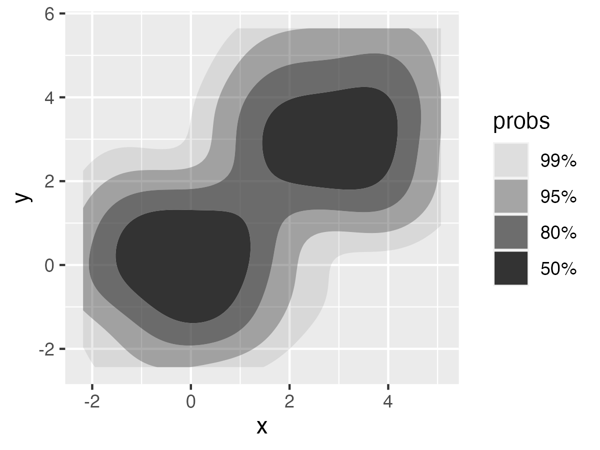
{densityarea} gives direct access to these HDRs, either
as data frames or as simple
features, for further analysis.
You can install {densityarea} from CRAN with:
install.packages("densityarea")Or you can install the development version from GitHub with:
# install.packages("devtools")
devtools::install_github("JoFrhwld/densityarea")The use case the package was initially developed for was for estimating vowel space areas.
library(densityarea)
library(dplyr)
library(tidyr)
library(sf)

data(s01)

# initial data processing

s01 |>
  mutate(lF1 = -log(F1),
         lF2 = -log(F2))->
  s01
To get this speaker’s vowel space area we can pass the data through
dplyr::reframe()
s01 |>
  reframe(
    density_area(lF2, lF1, probs = 0.8)
  )
#> # A tibble: 1 × 3
#>   level_id  prob  area
#>      <int> <dbl> <dbl>
#> 1        1   0.8 0.406
Or, we could get the spatial polygon associated with the 80% probability level
s01 |>
  reframe(
    density_polygons(lF2, lF1, probs = 0.8, as_sf = T)
  )
#> # A tibble: 1 × 3
#>   level_id  prob                                                        geometry
#>      <int> <dbl>                                                       <POLYGON>
#> 1        1   0.8 ((-7.777586 -6.009484, -7.801131 -6.010429, -7.824676 -6.01700…
For more details on using {densityarea}, see , and for
further information on using spatial polygons, see
vignette("sf-operations").
Otto J, Kahle D (2023). ggdensity: Interpretable Bivariate Density Visualization with ‘ggplot2’. https://jamesotto852.github.io/ggdensity/ https://github.com/jamesotto852/ggdensity/↩︎