![]()
![]()
![]()
![]()
This R package is a wrapper of the C++ library epiworld. It provides a general framework for modeling disease transmission using agent-based models. Some of the main features include:
From the package’s description:
A flexible framework for Agent-Based Models (ABM), the epiworldR package provides methods for prototyping disease outbreaks and transmission models using a C++ backend, making it very fast. It supports multiple epidemiological models, including the Susceptible-Infected-Susceptible (SIS), Susceptible-Infected-Removed (SIR), Susceptible-Exposed-Infected-Removed (SEIR), and others, involving arbitrary mitigation policies and multiple-disease models. Users can specify infectiousness/susceptibility rates as a function of agents’ features, providing great complexity for the model dynamics. Furthermore, epiworldR is ideal for simulation studies featuring large populations.
Current available models:
Note: Measles-specific models have been moved to the
separate measles R
package.
Note: Measles-specific models have been moved to the
separate measles R
package.
ModelDiagramModelDiffNetModelSEIRModelSEIRCONNModelSEIRDModelSEIRDCONNModelSEIRMixingModelSEIRMixingQuarantineModelSIRModelSIRCONNModelSIRDModelSIRDCONNModelSIRLogitModelSIRMixingModelSISModelSISDModelSURVYou can install the development version of epiworldR from GitHub with:
devtools::install_github("UofUEpiBio/epiworldR")Or from R-universe (recommended for the latest development version):
install.packages(
  'epiworldR',
  repos = c(
    'https://uofuepibio.r-universe.dev',
    'https://cloud.r-project.org'
  )
)
Or from CRAN
install.packages("epiworldR")This R package includes several popular epidemiological models, including SIS, SIR, and SEIR using either a fully connected graph (similar to a compartmental model) or a user-defined network.
This Susceptible-Infected-Recovered model features a population of 100,000 agents simulated in a small-world network. Each agent is connected to ten other agents. One percent of the population has the virus, with a 70% chance of transmission. Infected individuals recover at a 0.3 rate:
library(epiworldR)
#> Thank you for using epiworldR! Please consider citing it in your work.
#> You can find the citation information by running
#>   citation("epiworldR")

# Creating a SIR model
sir <- ModelSIR(
  name              = "COVID-19",
  prevalence        = .01,
  transmission_rate = .7,
  recovery          = .3
) |>
  # Adding a Small world population
  agents_smallworld(n = 100000, k = 10, d = FALSE, p = .01) |>
  # Running the model for 50 days
  run(ndays = 50, seed = 1912)
#> _________________________________________________________________________
#> |Running the model...
#> |||||||||||||||||||||||||||||||||||||||||||||||||||||||||||||||||||||||| done.
#> |

sir
#> ________________________________________________________________________________
#> Susceptible-Infected-Recovered (SIR)
#> It features 100000 agents, 1 virus(es), and 0 tool(s).
#> The model has 3 states.
#> The final distribution is: 0 Susceptible, 0 Infected, and 100000 Recovered.
Visualizing the outputs
summary(sir)
#> ________________________________________________________________________________
#> ________________________________________________________________________________
#> SIMULATION STUDY
#>
#> Name of the model   : Susceptible-Infected-Recovered (SIR)
#> Population size     : 100000
#> Agents' data        : (none)
#> Number of entities  : 0
#> Days (duration)     : 50 (of 50)
#> Number of viruses   : 1
#> Last run elapsed t  : 206.00ms
#> Last run speed      : 24.26 million agents x day / second
#> Rewiring            : off
#> Last seed used      : 1912
#>
#> Global events:
#>  (none)
#>
#> Virus(es):
#>  - COVID-19
#>
#> Tool(s):
#>  (none)
#>
#> Model parameters:
#>  - Recovery rate     : 0.3000
#>  - Transmission rate : 0.7000
#>
#> Distribution of the population at time 50:
#>   - (0) Susceptible :  99000 -> 0
#>   - (1) Infected    :   1000 -> 0
#>   - (2) Recovered   :      0 -> 100000
#>
#> Transition Probabilities:
#>  - Susceptible  0.85  0.15     -
#>  - Infected        -  0.70  0.30
#>  - Recovered       -     -  1.00
plot(sir)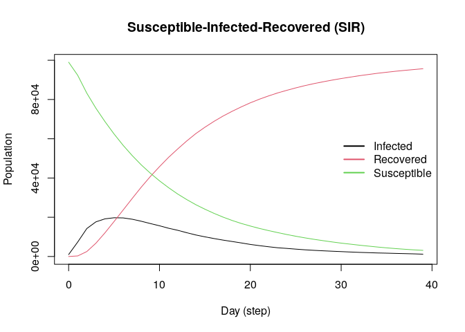
plot_incidence(sir)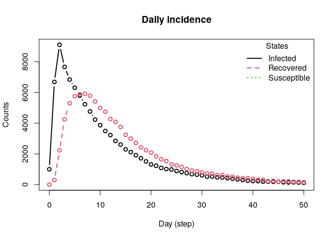
The SEIR model is similar to the SIR model but includes an exposed state. Here, we simulate a population of 10,000 agents with a 0.01 prevalence, a 0.6 transmission rate, a 0.5 recovery rate, and 7 days-incubation period. The population is fully connected, meaning agents can transmit the disease to any other agent:
model_seirconn <- ModelSEIRCONN(
  name                = "COVID-19",
  prevalence          = 0.01,
  n                   = 10000,
  contact_rate        = 10,
  incubation_days     = 7,
  transmission_rate   = 0.1,
  recovery_rate       = 1 / 7
) |> add_virus(
  virus(
    name = "COVID-19 (delta)",
    prevalence = 0.01,
    as_proportion = TRUE,
    prob_infecting = 0.2,
    recovery_rate = 0.6,
    prob_death = 0.5,
    incubation = 7
))

set.seed(132)
run(model_seirconn, ndays = 100)
#> _________________________________________________________________________
#> Running the model...
#> ||||||||||||||||||||||||||||||||||||||||||||||||||||||||||||||||||||||||| done.
summary(model_seirconn)
#> ________________________________________________________________________________
#> ________________________________________________________________________________
#> SIMULATION STUDY
#>
#> Name of the model   : Susceptible-Exposed-Infected-Removed (SEIR) (connected)
#> Population size     : 10000
#> Agents' data        : (none)
#> Number of entities  : 0
#> Days (duration)     : 100 (of 100)
#> Number of viruses   : 2
#> Last run elapsed t  : 28.00ms
#> Last run speed      : 35.65 million agents x day / second
#> Rewiring            : off
#> Last seed used      : 2587
#>
#> Global events:
#>  - Update infected individuals (runs daily)
#>
#> Virus(es):
#>  - COVID-19
#>  - COVID-19 (delta)
#>
#> Tool(s):
#>  (none)
#>
#> Model parameters:
#>  - Avg. Incubation days : 7.0000
#>  - Contact rate         : 10.0000
#>  - Prob. Recovery       : 0.1429
#>  - Prob. Transmission   : 0.1000
#>
#> Distribution of the population at time 100:
#>   - (0) Susceptible :  9800 -> 60
#>   - (1) Exposed     :   200 -> 0
#>   - (2) Infected    :     0 -> 0
#>   - (3) Recovered   :     0 -> 9940
#>
#> Transition Probabilities:
#>  - Susceptible  0.95  0.05     -     -
#>  - Exposed         -  0.86  0.14     -
#>  - Infected        -     -  0.78  0.22
#>  - Recovered       -     -     -  1.00
Computing some key statistics
plot(model_seirconn)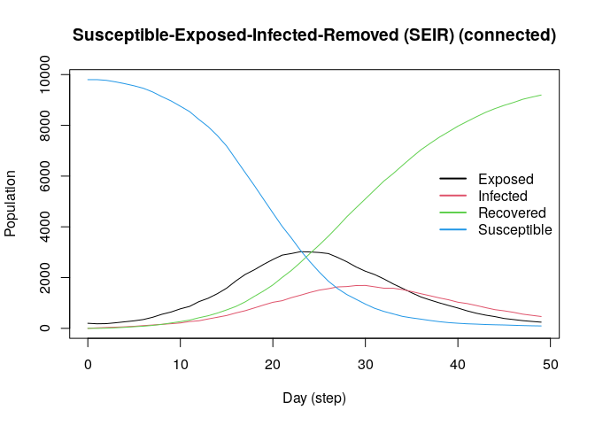
repnum <- get_reproductive_number(model_seirconn)

head(plot(repnum))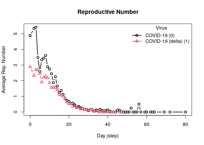
#>   virus_id    virus date      avg   n       sd lb     ub
#> 1        0 COVID-19    0 4.980000 100 4.442631  0 15.525
#> 2        0 COVID-19    2 2.818182  11 2.638870  0  7.500
#> 3        0 COVID-19    3 4.285714  21 4.112698  0 13.500
#> 4        0 COVID-19    4 4.520000  25 3.809199  0 12.200
#> 5        0 COVID-19    5 3.363636  33 2.859394  0  9.000
#> 6        0 COVID-19    6 3.961538  52 2.976783  0 10.000

head(plot_generation_time(model_seirconn))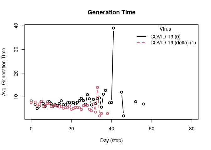
#>   date      avg  n       sd ci_lower ci_upper    virus virus_id
#> 1    0 7.788889 90 5.042503    2.000   18.550 COVID-19        0
#> 2    2 9.333333  9 5.916080    2.400   19.600 COVID-19        0
#> 3    3 9.000000 18 8.116794    2.000   27.375 COVID-19        0
#> 4    4 6.523810 21 3.776494    2.000   14.500 COVID-19        0
#> 5    5 8.666667 27 6.120583    2.000   22.750 COVID-19        0
#> 6 6 6.727273 44 4.576805 2.075 17.925 COVID-19 0This model provides a more complex transmission and recovery pattern
based on agents’ features. With it, we can reflect co-morbidities that
could change the probability of infection and recovery. Here, we
simulate a population including a dataset with two features: an
intercept and a binary variable Female. The probability of
infection and recovery are functions of the intercept and the
Female variables. The following code simulates a population
of 100,000 agents in a small-world network. Each agent is connected to
eight other agents. One percent of the population has the virus, with an
80% chance of transmission. Infected individuals recover at a 0.3
rate:
# Simulating a population of 100,000 agents
set.seed(2223)
n <- 100000

# Agents' features
X <- cbind(
  Intercept = 1,
  Female    = sample.int(2, n, replace = TRUE) - 1
)

coef_infect  <- c(.1, -2, 2)
coef_recover <- rnorm(2)

# Creating the model
model_logit <- ModelSIRLogit(
  "covid2",
  data = X,
  coefs_infect      = coef_infect,
  coefs_recover     = coef_recover,
  coef_infect_cols  = 1L:ncol(X),
  coef_recover_cols = 1L:ncol(X),
  prob_infection = .8,
  recovery_rate = .3,
  prevalence = .01
)

# Adding a small-world population
agents_smallworld(model_logit, n, 8, FALSE, .01)

# Running the model
run(model_logit, 50)
#> _________________________________________________________________________
#> |Running the model...
#> |||||||||||||||||||||||||||||||||||||||||||||||||||||||||||||||||||||||| done.
#> |
plot(model_logit)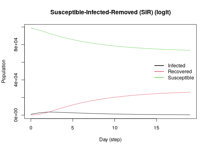
# Females are supposed to be more likely to become infected
rn <- get_reproductive_number(model_logit)

(table(
  X[, "Female"],
  (1:n %in% rn$source)
) |> prop.table())[, 2]
#>       0       1
#> 0.20317 0.21753

# Looking into the agents
get_agents(model_logit)
#> Agents from the model "Susceptible-Infected-Removed (SIR) (logit)":
#> Agent: 1, state: Susceptible (0), Has virus: no, NTools: 0i NNeigh: 8
#> Agent: 2, state: Susceptible (0), Has virus: no, NTools: 0i NNeigh: 8
#> Agent: 3, state: Susceptible (0), Has virus: no, NTools: 0i NNeigh: 8
#> Agent: 4, state: Susceptible (0), Has virus: no, NTools: 0i NNeigh: 8
#> Agent: 5, state: Susceptible (0), Has virus: no, NTools: 0i NNeigh: 8
#> Agent: 6, state: Susceptible (0), Has virus: no, NTools: 0i NNeigh: 8
#> Agent: 7, state: Susceptible (0), Has virus: no, NTools: 0i NNeigh: 8
#> Agent: 8, state: Susceptible (0), Has virus: no, NTools: 0i NNeigh: 8
#> Agent: 9, state: Susceptible (0), Has virus: no, NTools: 0i NNeigh: 8
#> Agent: 10, state: Susceptible (0), Has virus: no, NTools: 0i NNeigh: 8
#> ... 99990 more agents ...This example shows how we can draw a transmission network from a simulation. The following code simulates a population of 500 agents in a small-world network. Each agent is connected to ten other agents. One percent of the population has the virus, with a 50% chance of transmission. Infected individuals recover at a 0.5 rate:
# Creating a SIR model
sir <- ModelSIR(
  name           = "COVID-19",
  prevalence     = .01,
  transmission_rate = .5,
  recovery       = .5
) |>
  # Adding a Small world population
  agents_smallworld(n = 500, k = 10, d = FALSE, p = .01) |>
  # Running the model for 50 days
  run(ndays = 50, seed = 1912)
#> _________________________________________________________________________
#> |Running the model...
#> |||||||||||||||||||||||||||||||||||||||||||||||||||||||||||||||||||||||| done.
#> |

# Transmission network
net <- get_transmissions(sir)
net <- subset(net, source >= 0)

# Plotting
library(epiworldR)
library(netplot)
#> Loading required package: grid
x <- igraph::graph_from_edgelist(
  as.matrix(net[, 2:3]) + 1
)

nplot(x, edge.curvature = 0, edge.color = "gray", skip.vertex = TRUE)![]()
epiworldR supports running multiple simulations using
the run_multiple function. The following code simulates 50
SIR models with 1000 agents each. Each agent is connected to ten other
agents. One percent of the population has the virus, with a 90% chance
of transmission. Infected individuals recover at a 0.1 rate. The results
are saved in a data.frame:
model_sir <- ModelSIRCONN(
  name = "COVID-19",
  prevalence = 0.01,
  n = 1000,
  contact_rate = 2,
  transmission_rate = 0.9, recovery_rate = 0.1
)

# Generating a saver
saver <- make_saver("total_hist", "reproductive")

# Running and printing
# Notice the use of nthread = 2 to run the simulations in parallel
run_multiple(model_sir, ndays = 100, nsims = 50, saver = saver, nthread = 2)
#> Starting multiple runs (50) using 2 thread(s)
#> _________________________________________________________________________
#> _________________________________________________________________________
#> ||||||||||||||||||||||||||||||||||||||||||||||||||||||||||||||||||||||||| done.

# Retrieving the results
ans <- run_multiple_get_results(model_sir)

head(ans$total_hist)
#>   sim_num date nviruses       state counts
#> 1       1    0        1 Susceptible    990
#> 2       1    0        1    Infected     10
#> 3       1    0        1   Recovered      0
#> 4       1    1        1 Susceptible    967
#> 5       1    1        1    Infected     33
#> 6       1    1        1   Recovered      0
head(ans$reproductive)
#>   sim_num virus_id    virus source source_exposure_date rt
#> 1       1        0 COVID-19    855                   10  0
#> 2       1        0 COVID-19    427                   10  0
#> 3       1        0 COVID-19    577                    9  0
#> 4       1        0 COVID-19    951                    8  1
#> 5       1        0 COVID-19    783                    8  0
#> 6       1        0 COVID-19    778                    8  0

plot(ans$reproductive)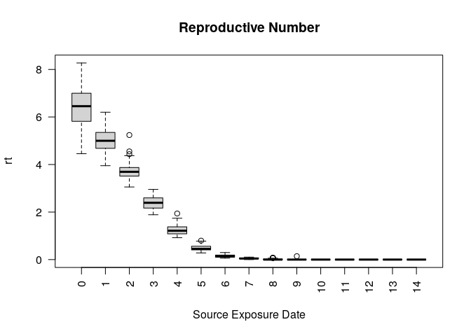
The virtual INSNA Sunbelt 2023 session can be found here: https://github.com/UofUEpiBio/epiworldR-workshop/tree/sunbelt2023-virtual
The in-person INSNA Sunbelt 2023 session can be found here: https://github.com/UofUEpiBio/epiworldR-workshop/tree/sunbetl2023-inperson
If you use epiworldR in your research, please cite it as
follows:
citation("epiworldR")
#> To cite epiworldR in publications use:
#>
#>   Meyer, Derek and Vega Yon, George (2023). epiworldR: Fast Agent-Based
#>   Epi Models. Journal of Open Source Software, 8(90), 5781,
#>   https://doi.org/10.21105/joss.05781
#>
#> And the actual R package:
#>
#>   Meyer D, Pulsipher A, Vega Yon G (2025). _epiworldR: Fast Agent-Based
#>   Epi Models_. R package version 0.14.0.0,
#>   <https://github.com/UofUEpiBio/epiworldR>.
#>
#> To see these entries in BibTeX format, use 'print(<citation>,
#> bibtex=TRUE)', 'toBibtex(.)', or set
#> 'options(citation.bibtex.max=999)'.Several alternatives to epiworldR exist and provide
researchers with a range of options, each with its own unique features
and strengths, enabling the exploration and analysis of infectious
disease dynamics through agent-based modeling. Below is a manually
curated table of existing alternatives, including ABM [@ABM], abmR [@abmR], cystiSim [@cystiSim], villager
[@villager], and
RNetLogo [@RNetLogo].
| Package | Multiple Viruses | Multiple Tools | Multiple Runs | Global Actions | Built-In Epi Models | Dependencies | Activity |
|---|---|---|---|---|---|---|---|
| epiworldR | yes | yes | yes | yes | yes |  |
|
| ABM | - | - | - | yes | yes |  |
|
| abmR | - | - | yes | - | - |  |
|
| cystiSim | - | yes | yes | - | - |  |
|
| villager | - | - | - | yes | - |  |
|
| RNetLogo | - | yes | yes | yes | - |  |
You may want to check out other R packages for agent-based modeling:
ABM,
abmR,
cystiSim,
villager, and
RNetLogo.
We welcome contributions to the epiworldR package! If you would like to contribute, please review our development guidelines before creating a pull request.
The epiworldR project is released with a Contributor Code of Conduct. By contributing to this project, you agree to abide by its terms.