![]()
![]()
Welcome to the SkipTrack Package!
SkipTrack is a Bayesian hierarchical model for self-reported menstrual cycle length data on mobile health apps. The model is an extension of the hierarchical model presented in Li et al. (2022) that focuses on predicting an individual’s next menstrual cycle start date while accounting for cycle length inaccuracies introduced by non-adherence in user self-tracked data. Check out the ‘Getting Started’ vignette to see an overview of the SkipTrack Model!
#Install from CRAN
install.packages('skipTrack')

#Install Development Version
devtools::install_github("LukeDuttweiler/skipTrack")The SkipTrack package provides functions for fitting the SkipTrack model, evaluating model run diagnostics, retrieving and visualizing model results, and simulating related data. We begin our tutorial by examining some simulated data.
library(skipTrack)First, we simulate data on 100 individuals from the SkipTrack model where each observed \(y_{ij}\) value has a 75% probability of being a true cycle, a 20% probability of being two true cycles recorded as one, and a 5% probability of being three true cycles recorded as one.
set.seed(1)

#Simulate data
dat <- skipTrack.simulate(n = 100, model = 'skipTrack', skipProb = c(.75, .2, .05))
Fitting the SkipTrack model using this simulated data requires a call
to the function skipTrack.fit. Note that because this is a
Bayesian model and is fit with an MCMC algorithm, it can take some time
with large datasets and a high number of MCMC reps and chains.
In this code we ask for 4 chains, each with 1000 iterations, run sequentially. Note that we recommend allowing the sampler to run longer than this (usually at least 5000 iterations per chain), but we use a short run here to save time.
If useParallel = TRUE, the MCMC chains will be evaluated
in parallel, which helps with longer runs.
ft <- skipTrack.fit(Y = dat$Y, cluster = dat$cluster,
                    reps = 1000, chains = 4, useParallel = FALSE)
Once we have the model results we are able to examine model diagnostics, visualize results from the model, and view a model summary.
Multivariate, multichain MCMC diagnostics, including traceplots,
Gelman-Rubin diagnostics, and effective sample size, are all available
for various parameters from the model fit. These are supplied using the
genMCMCDiag package, see that packages’ documentation for
details.
Here we show the output of the diagnostics on the \(c_{ij}\) parameters, which show that (at least for the \(c_{ij}\) values) the algorithm is mixing effectively (or will be, once the algorithm runs a little longer).
skipTrack.diagnostics(ft, param = 'cijs')
#> Warning in attr(x, "align"): 'xfun::attr()' is deprecated.
#> Use 'xfun::attr2()' instead.
#> See help("Deprecated")
#> Warning in attr(x, "align"): 'xfun::attr()' is deprecated.
#> Use 'xfun::attr2()' instead.
#> See help("Deprecated")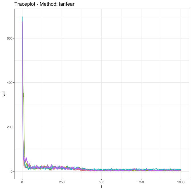
#> ----------------------------------------------------
#> Generalized MCMC Diagnostics using Custom Method
#> ----------------------------------------------------
#>
#> |Effective Sample Size:
#> |---------------------------
#> | Chain 1| Chain 2| Chain 3| Chain 4|    Sum|
#> |-------:|-------:|-------:|-------:|------:|
#> |  26.895|  18.342|  18.723|  19.814| 83.774|
#>
#> |psrf:
#> |---------------------------
#> | Point est.| Upper C.I.|
#> |----------:|----------:|
#> | 1.003| 1.009|In order to see some important plots for the SkipTrack model fit, you
can simply use plot(ft), and the plots are directly
accessible using skipTrack.visualize(ft).
plot(ft)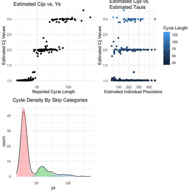
A summary is available for the SkipTrack model fit with
summary(ft), with more detailed results accessible through
skipTrack.results(ft). Importantly, these results are based
on a default chain burn-in value of 750 draws. This can be changed using
the parameter burnIn for either function.
For example using summary with the default burnIn…
summary(ft)produces the following output:
#> ----------------------------------------------------
#> Summary of skipTrack.fit using skipTrack model
#> ----------------------------------------------------
#> Mean Coefficients:
#>
#>             Estimate       95% CI Lower 95% CI Upper
#> (Intercept)    3.406              3.382        3.437
#>
#> ----------------------------------------------------
#> Precision Coefficients:
#>
#>             Estimate       95% CI Lower 95% CI Upper
#> (Intercept)    5.342              5.156         5.53
#>
#> ----------------------------------------------------
#> Diagnostics:
#>
#>        Effective Sample Size       Gelman-Rubin
#> Betas                3077.74               1.00
#> Gammas                 21.85               1.01
#> cijs                   68.15               1.00
#>
#> ----------------------------------------------------
On the other hand if we change the burnIn to 500…
summary(ft, burnIn = 500)we see:
#> ----------------------------------------------------
#> Summary of skipTrack.fit using skipTrack model
#> ----------------------------------------------------
#> Mean Coefficients:
#>
#>             Estimate       95% CI Lower 95% CI Upper
#> (Intercept)    3.405              3.378        3.433
#>
#> ----------------------------------------------------
#> Precision Coefficients:
#>
#>             Estimate       95% CI Lower 95% CI Upper
#> (Intercept)    5.322              5.106        5.526
#>
#> ----------------------------------------------------
#> Diagnostics:
#>
#>        Effective Sample Size       Gelman-Rubin
#> Betas                3818.63               1.00
#> Gammas                 22.59               1.01
#> cijs                   75.03               1.01
#>
#> ----------------------------------------------------
This introduction provides enough information to start fitting the SkipTrack model. For further information regarding different methods of simulating data, additional model fitting, and tuning parameters for fitting the model, please see the help pages and the ‘Getting Started’ vignette. Additional vignettes are forthcoming.